Entry 12
Authors
- Kristen Thyng
- Rob Hetland
The circulation of the waters on the Texas and Louisiana continental shelf is complex and dynamic. Many of the applications of understanding the circulation are related to how material in a region, like spilled oil or a harmful algal bloom, is transported by the currents. This transport can be investigated using drifters, which are passively moved by the ocean currents.
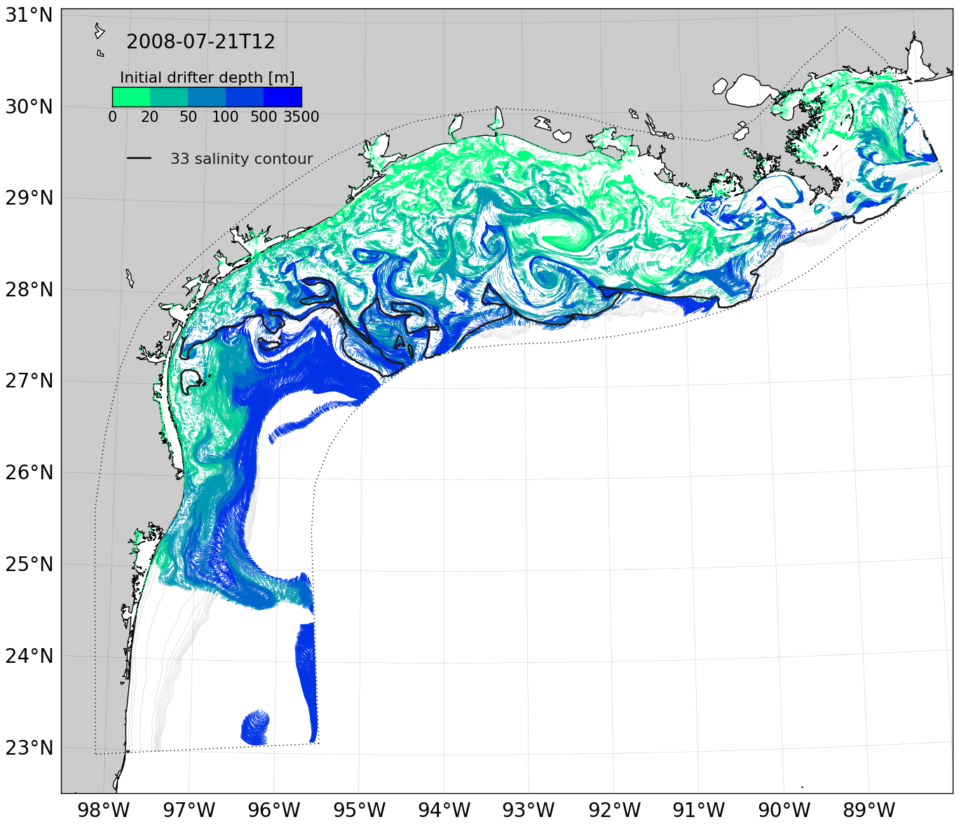
This animation shows simulated drifters (with short tails showing a time history) at the sea surface of a numerical model of the currents on the Texas and Louisiana shelf. The drifters are started uniformly throughout the model domain. The released drifters immediately demonstrate the complexity of the underlying flow fields: drifters offshore near the outer model edge generally move together while drifters nearer the mouths of the Mississippi and Atchafalaya rivers form filaments due to convergence and divergence associated with eddies along the edge of the river plume. These eddies are seen within the river plume, the extent of which is marked by a solid black line.
The drifters are colored by the water column depth of their starting location. As the drifters evolve in time, they sometimes move on- or off-shore, as seen by greener drifters found farther from, and bluer drifters nearer to, the coast. This represents cross-shelf movement and is a means by which off-shore oil spills can move toward the shore, or by which river-borne materials can leave the shelf toward deeper waters. The regular circular “jiggling” of the drifters is not due to tides, but rather inertial oscillations in the flow field: the regular land/sea breeze due to heating and cooling of the land during the day and at night aligns with the approximately 24-hour period of particle motion due to the Coriolis effect near 30˚ latitude. Visualizations of drifter motion in time allows for better understanding of important transport processes in this region.
Source
'''
Plot a set of drifters in map view, in time.
'''

import matplotlib.pyplot as plt
import netCDF4 as netCDF
import tracpy
import tracpy.plotting
from matplotlib.mlab import find
import pdb
import numpy as np
import matplotlib as mpl
import os
import tracpy.calcs
import glob
from datetime import datetime, timedelta

mpl.rcParams.update({'font.size': 20})
mpl.rcParams['font.sans-serif'] = 'Arev Sans, Bitstream Vera Sans, Lucida Grande, Verdana, Geneva, Lucid, Helvetica, Avant Garde, sans-serif'
mpl.rcParams['mathtext.fontset'] = 'custom'
mpl.rcParams['mathtext.cal'] = 'cursive'
mpl.rcParams['mathtext.rm'] = 'sans'
mpl.rcParams['mathtext.tt'] = 'monospace'
mpl.rcParams['mathtext.it'] = 'sans:italic'
mpl.rcParams['mathtext.bf'] = 'sans:bold'
mpl.rcParams['mathtext.sf'] = 'sans'
mpl.rcParams['mathtext.fallback_to_cm'] = 'True'

# read in grid
# loc = 'http://barataria.tamu.edu:6060/thredds/dodsC/NcML/txla_nesting6.nc'
# loc = '/atch/raid1/zhangxq/Projects/txla_nesting6/txla_grd_v4_new.nc'
loc = 'grid.nc'
grid = tracpy.inout.readgrid(loc, usebasemap=True)

# Read in drifter tracks
dd = 1 # 500 # drifter decimation

## This is how to retrieve the output from the (2GB) file ##
startdate = '2008-07-15T00' #4'
# d = netCDF.Dataset('tracks/' + startdate + 'gc.nc')
# xg = d.variables['xg'][::dd,:]
# yg = d.variables['yg'][::dd,:]
# ind = (xg == -1)
# xp, yp, _ = tracpy.tools.interpolate2d(xg, yg, grid, 'm_ij2xy')
# xp[ind] = np.nan; yp[ind] = np.nan
# if d.variables['tp'].ndim == 1:
#     tp = d.variables['tp'][:]
# elif d.variables['tp'].ndim > 1:
#     # index of a drifter that lasts the whole time
#     itp = np.argmax(np.max(d.variables['tp'][:], axis=1))
#     tp = d.variables['tp'][itp,:]

# units = d.variables['tp'].units
####

# days = (tp-tp[0])/(3600.*24)
# dates = netCDF.num2date(tp, units)
days = np.arange(0,16,(4./24))
dates = []
[dates.append(datetime(2008,07,15,0,0) + timedelta(hours=4*i)) for i in xrange(96)]

## Fake data ##
# have a drifter at every few grid cells
xp = grid['xr'][::10,::10].flatten(); yp = grid['yr'][::10,::10].flatten()
xp = xp[:,np.newaxis].repeat(days.size, axis=1)
yp = yp[:,np.newaxis].repeat(days.size, axis=1)
xp += 1000*np.random.randn(*xp.shape)
yp += 1000*np.random.randn(*yp.shape)
h = grid['h']
# txla output
## Model output ##
## don't use real data since too big ##
# currents_filenames = loc
# nc = netCDF.Dataset(currents_filenames)
# datestxla = netCDF.num2date(nc.variables['ocean_time'][:], nc.variables['ocean_time'].units)
####

# Find indices of drifters by starting depth
# depthp = tracpy.calcs.Var(xg[:,0], yg[:,0], nc, 'h', nc) # starting depths of drifters
# near-shore
# ind10 = depthp<=10
ind20 = (h[::10,::10]<=20).flatten()
ind50 = ((h[::10,::10]>20)*(h[::10,::10]<=50)).flatten()
ind100 = ((h[::10,::10]>50)*(h[::10,::10]<=100)).flatten()
# offshore
ind500 = ((h[::10,::10]>100)*(h[::10,::10]<=500)).flatten()
ind3500 = (h[::10,::10]>500).flatten()

# colors for drifters
rgb = plt.cm.get_cmap('winter_r')(np.linspace(0,1,6))[:-1,:3] # skip last entry where it levels off in lightness

# to plot colorbar
gradient = np.linspace(0, 1, 6)[:-1]
gradient = np.vstack((gradient, gradient))

ms = 1.5 # markersize

# make fake salt data
salt = grid['h'].T

# Plot drifters, starting 5 days into simulation
# 2 days for one tail, 3 days for other tail
# Find indices relative to present time
i5daysago = 0 # keeps track of index 5 days ago
i2daysago = find(days>=3)[0] # index for 2 days ago, which starts as 3 days in
i5days = 0 # start at the beginning
nt = days.size # total number of time indices

dirname = 'figures/drifters/dd' + str(dd) + '/' + startdate

for i in np.arange(i5days,nt+1,5):

    fname = dirname + '/' + dates[i].isoformat()[:-6] + '.png'

    ## don't actually read in model output each step, use fake instead ##
    # itxla = np.where(datestxla==dates[i])[0][0] # find time index to use for model output
    # salt = nc.variables['salt'][itxla,-1,:,:] # surface salinity
    ####

    # Plot background
    fig = plt.figure(figsize=(18,14))
    ax = fig.add_subplot(111)
    tracpy.plotting.background(grid=grid, ax=ax)

    istart = i-(24./3*4*0.25) # when to start plotting lines back in time
    if istart<0: istart=0

    if i==0:

        # Plot drifter locations
        ax.plot(xp[ind20,i].T, yp[ind20,i].T, 'o', color=rgb[0,:], ms=0.6, mec='None')
        ax.plot(xp[ind50,i].T, yp[ind50,i].T, 'o', color=rgb[1,:], ms=0.6, mec='None')
        ax.plot(xp[ind100,i].T, yp[ind100,i].T, 'o', color=rgb[2,:], ms=0.6, mec='None')
        ax.plot(xp[ind500,i].T, yp[ind500,i].T, 'o', color=rgb[3,:], ms=0.6, mec='None')
        ax.plot(xp[ind3500,i].T, yp[ind3500,i].T, 'o', color=rgb[4,:], ms=0.6, mec='None')

    else:

        # Plot drifter locations
        ax.plot(xp[ind20,istart:i+1].T, yp[ind20,istart:i+1].T, '-', color=rgb[0,:], lw=0.5)
        ax.plot(xp[ind50,istart:i+1].T, yp[ind50,istart:i+1].T, '-', color=rgb[1,:], lw=0.5)
        ax.plot(xp[ind100,istart:i+1].T, yp[ind100,istart:i+1].T, '-', color=rgb[2,:], lw=0.5)
        ax.plot(xp[ind500,istart:i+1].T, yp[ind500,istart:i+1].T, '-', color=rgb[3,:], lw=0.5)
        ax.plot(xp[ind3500,istart:i+1].T, yp[ind3500,istart:i+1].T, '-', color=rgb[4,:], lw=0.5)

    # Overlay surface salinity
    # pdb.set_trace()
    ax.contour(grid['xr'].T, grid['yr'].T, salt, [33], colors='0.1', zorder=12, linewidths=2)

    # Time
    ax.text(0.075, 0.95, dates[i].isoformat()[:-6], transform=ax.transAxes, fontsize=20)

    # Drifter legend
    cax = fig.add_axes([0.2, 0.8, 0.15, 0.02])
    cax.imshow(gradient, aspect='auto', interpolation='none', cmap=plt.get_cmap('winter_r'))
    cax.tick_params(axis='y', labelleft=False, left=False, right=False)
    cax.tick_params(axis='x', top=False, bottom=False, labelsize=15)
    cax.set_xticks(np.arange(-0.5, 5, 1.0))
    cax.set_xticklabels(('0', '20', '50', '100', '500', '3500'))
    cax.set_title('Initial drifter depth [m]', fontsize=16)
    # legend for contour
    ax.plot([0.075, 0.1], [0.81, 0.81], '0.1', lw=2, transform=ax.transAxes)
    ax.text(0.123, 0.802, '33 salinity contour', color='0.1', transform=ax.transAxes, fontsize=16)

    # Update indices
    i5daysago += 5
    i2daysago += 5

    # Don't save for this example case
    # fig.savefig(fname, bbox_inches='tight')

    plt.close()

# Use ffmpeg to make images together