Entry 13

Video

Authors

• Haifeng Yang

How stars are formed is one of the big questions in astronomy. Answering this question helps us to understand the origin of our solar system. Currently people believe there to be proto-stellar disks around the forming stars. On the other hand, moderate magnetic field was observed in molecular clouds, where stars are forming. However, these two facts kind of conflict each other. A magnetized cloud will concentrate the magnetic field lines as it collapses and eventually introduce a big torque to the rotation supported disk. A moderately strong magnetic field is enough to prevent a disk from forming. This is called magnetic braking catastrophe and is still an open question to answer.

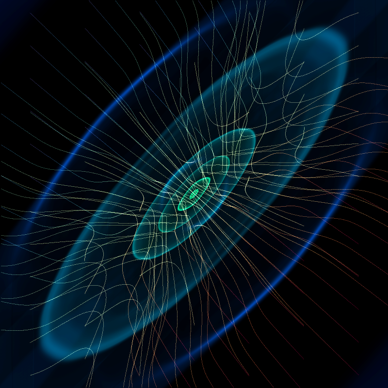
Numerical simulation is one way to address such problems. This visualization comes from a magnetic hydrodynamic simulation done with Adaptive-Mesh-Refinement code ENZO. Constrain Transfer method was applied to clean up the divergence of magnetic field and the star is treated as a sink particle in this simulation. Under the help of yt, I am able to show the density contour together with the magnetic field lines. A single color map is applied for density contour for all frames. The appearance of denser part after several frames shows the accretion of matter. The magnetic field lines are colored by the height, a.k.a. the \(z\) coordinate, to give a sense of spacial depth. We can see as the matter starts to concentrate, the magnetic field lines start to pinch heavily towards the center. This is typical in star formation and may lead to reconnection, which is essential in understanding and solving magnetic braking catastrophe.

This visualization goes through 26 frames of the simulation and span a time of 4200 years. After reaching the last frame, 72 more images were rendered showing the rotation of viewing angle. After the rendering of images, Sam Skillman’s script was applied to fix the brightness.

Products

• Video

Source

import yt
from yt.visualization.api import Streamlines
import numpy as np
import sys

def streaming(ds, output="stream.npy", N = 8, scale = 0.03, toplot=False, c = np.array([0.5]*3)):
  """
  Calculate the streamlines of magnetic field given YTDataSet. 
  N is number of points in each direction. These points are the starting points of the streamlines.
  If toplot = True, a 3D matplotlib figure will be created and shown with all the streamlines.
  """
  print >>sys.stderr, "Working on : ", output
  mi, ma = 0.5-scale/2.0, 0.5+scale/2.0

  # The following part calculate the starting points for streamlines.
  x=np.linspace(mi, ma, N)
  y=np.linspace(mi, ma, N)
  z=np.linspace(mi, ma, N)
  xx,yy,zz=np.meshgrid(x,y,z)
  xx.shape=N**3
  yy.shape=N**3
  zz.shape=N**3
  inside=False
  if not inside:
    # Only points on the edges
    ind = (xx == mi) + (xx == ma) + (yy == mi) + (yy == ma) + (zz == mi) + (zz == ma) 
    M = sum(ind)
    xx=xx[ind]
    yy=yy[ind]
    zz=zz[ind]
    pos = np.zeros((M,3))
  else:
    # All N**3 points
    pos = np.zeros((N**3,3))
  pos[:,0] = xx
  pos[:,1] = yy
  pos[:,2] = zz
  periodicity = ds.periodicity
  ds.periodicity = (True, True, True) # yt streamline currently only work with periodic data. This is one way to fool it.
  
  streamlines = Streamlines(ds,pos,'Bx', 'By', 'Bz', length=scale*2)
  streamlines.integrate_through_volume()
  
  if output!= None:
    np.save(output, streamlines.streamlines)
  if toplot:
    import matplotlib.pylab as pl
    from mpl_toolkits.mplot3d import Axes3D
    fig=pl.figure()
    ax = Axes3D(fig)
    for stream in streamlines.streamlines:
      stream = stream[np.all(stream != 0.0, axis=1)]
      Bx, By, Bz = stream[:,0], stream[:,1], stream[:,2]
      ind = (Bx>mi) * (Bx<ma) * (By>mi) * (By<ma) * (Bz>mi) * (Bz<ma) 
      Bx=Bx[ind]
      By=By[ind]
      Bz=Bz[ind]
      ax.plot3D(Bx, By, Bz, alpha=0.3, color='b')
    ax.axis(xmin=mi,xmax=ma,ymin=mi,ymax=ma)
    ax.set_zlim(bottom=mi,top=ma)
    ax.set_xlabel("x")
    ax.set_ylabel("y")
    ax.set_zlabel("z")
    pl.show()
  
  ds.periodicity = periodicity # Change periodicity back just in case.

import yt
import numpy as np
from matplotlib import cm
import sys

def draw_line(cam, output, scale=0.03, ipf = "stream.npy"):
  """
  Make a snapshot given the camera. Load streamlines from ipf and draw them onto the image.
  """
  streamlines = np.load(ipf) 

  im = cam.snapshot()
  
  maxa = im[:,:,:3].sum(axis=2).max()
  cmap = cm.Spectral # Color map applied to draw lines.
  
  mi, ma = 0.5-scale/2.0, 0.5+scale/2.0
  
  count = 0
  for stream in streamlines:
    stream = stream[np.all(stream != 0.0, axis=1)]
    Bx, By, Bz = stream[:,0], stream[:,1], stream[:,2]
    # Only lines within the region we consider will be drawn onto the image
    ind = (Bx>mi) * (Bx<ma) * (By>mi) * (By<ma) * (Bz>mi) * (Bz<ma)
    Bx=Bx[ind]
    By=By[ind]
    Bz=Bz[ind]
    
    for i in range(len(Bx)-1):
      x1, y1, z1 = Bx[i], By[i], Bz[i]
      x2, y2, z2 = Bx[i+1], By[i+1], Bz[i+1]
      # The color of the line is based on the z value, a.k.a. the height. 
      z0 = 0.5*(z1+z2)
      bcolor = np.array(cmap((z0-mi)/scale)) * 0.025 # Multiply 0.025 so that the lines don't overwhelm the brightness.
      cam.draw_line(im, np.array([x1, y1, z1]), np.array([x2, y2, z2]), color = bcolor)
  
    count += 1
  
  print >>sys.stderr, 'About to write: ', output

  # Write the image to output
  yt.write_bitmap(im, output)

• Data for last frame