Entry 15

Authors

• Anna Bilous

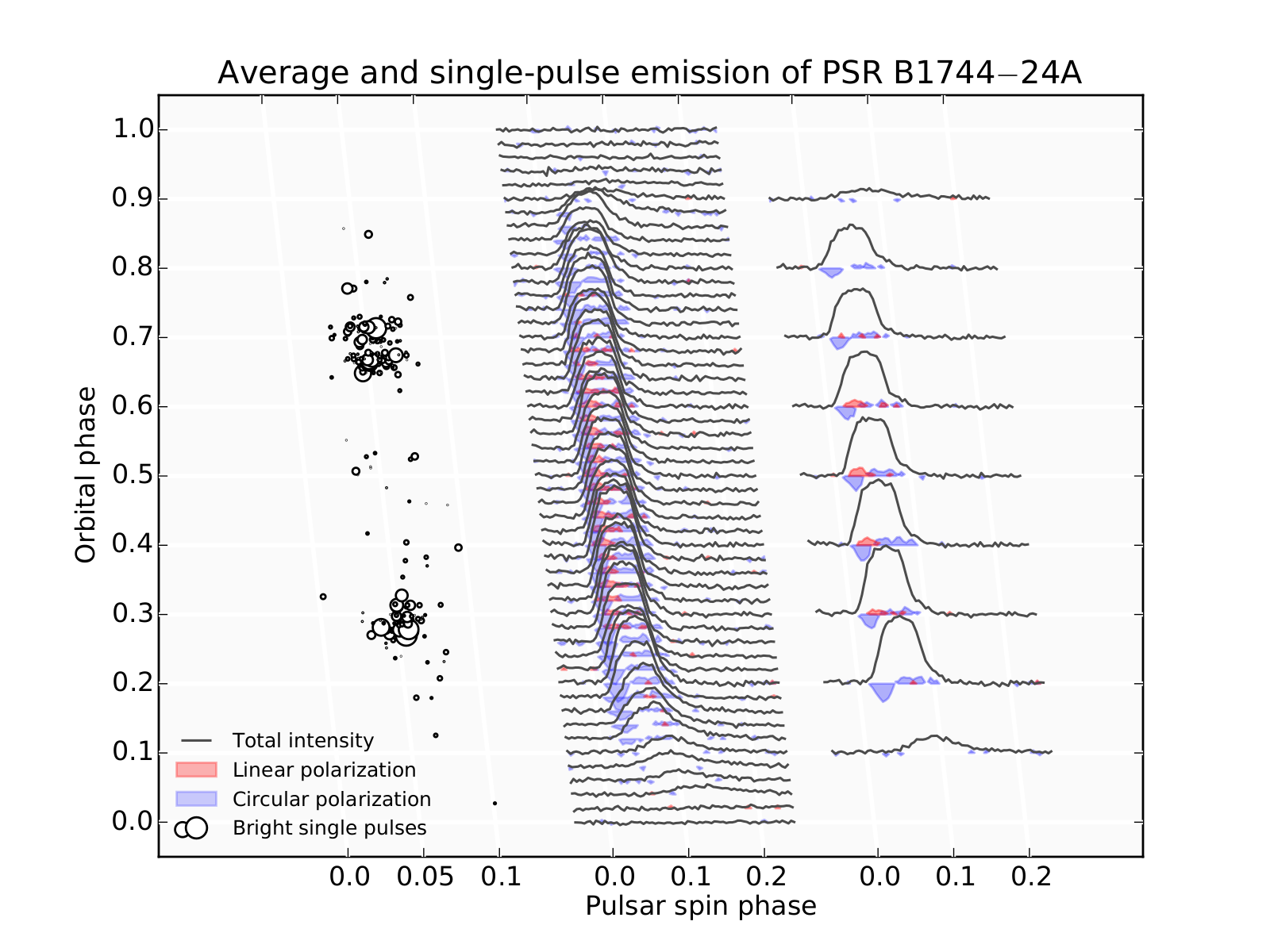
Average and single­pulse emission of PSR B1744–24A

Pulsars are one of the most exotic type of stars ever to be identified: they are born in supernova explosions, when a dying star leaves behind its rapidly spinning core, compressed to super-nuclear densities. Astonishingly small by astronomical scales (10-20 km), pulsars harbour ultra-strong magnetic fields and most of the time the only way to see them is to catch the narrow beam of electromagnetic radiation created by relativistic plasma in the pulsar’s magnetosphere. When this beam sweeps past the Earth, like the light from a lighthouse, a pulse is detected. The thorough investigation of these pulses provides a wealth of astrophysical information and can even be used to test fundamental physical theories.

PSR B1744–24A (also known as Ter5A) was the first pulsar discovered in globular cluster Terzan 5, a gravitationally bound agglomeration of stars that orbits Galactic core as a satellite. Similarly to many other pulsars, Ter5A at most times is too faint to be detected via individual pulses. However, the periodicity in incoming signal can be assessed by indirect methods and once the spin period of a pulsar is identified, so­called “average pulse” can be accumulated by folding the data stream synchronously with the spin period. The case of Ter5A is further complicated by the fact that the pulsar belongs to a tight binary system and the appearance of the average pulse is sometimes affected by the propagation through the cloud of plasma which surrounds the pulsar’s companion. The center part of the plot shows the evolution of the average pulse at radio wavelengths throughout one orbit. At the orbital phases 0.0 – 0.1 and 0.9 – 1.0 the pulsar is eclipsed by its companion and close to eclipses the propagation through the outer layers of companion star smears and delays observed pulses.

Ter5A emission poses few questions which still await their answers. One of them is the behaviour of linear polarization. In the middle of orbital period, where pulsar is in front of the companion and the pulsar radiation travels uninterrupted, the pulsar radio emission has moderate, but distinct level of linear polarization (see the inset on the right side with average pulses from selected orbital phases). Interestingly enough, this linearly polarized emission vanished in the vicinity of eclipses, but well before the shape of profile or level of circular polarization changes. Even more puzzling, there have been spotted bursts of strong pulses (shown on the left) which frame the disappearance of linear polarization. These pulses are so strong that we can detect them in original data, without any averaging. However, the fraction of such super-pulses is tiny and they do not influence the average intensity or pulse shape. It is currently unclear what makes these pulses so bright and how they are connected to the disappearance of the linear polarization in the average emission. We hope that investigating this will shed some light on the interaction of pulsar emission with companion’s plasma and the conditions in the binary system.

Products

• PDF

Source

import matplotlib.pyplot as plt
import numpy as np
import matplotlib.lines as mlines
import skew_projection


#==========================
# Loading data
#==========================

AP = np.load("Average_emission.npy")

I_AP = AP[0, 1:, 1:]  # Total intensity
L_AP = AP[1, 1:, 1:]  # Linearly polarized emission	
V_AP = AP[2, 1:, 1:]  # Circularly polarized emission
ph_spin_AP = AP[0, 0, 1:] # Spin phase of each emission sample
ph_orb_AP = AP[0, 1:, 0]  # Orbital phase of each emission sample

# Loading orbital phase, spin phase and energy of single pulses
ph_orb_SP, ph_spin_SP, E_SP = np.loadtxt("Single_pulses.txt", usecols=(0,1,2), unpack=True, dtype=float)

Nsub = len(AP[0, 1:, 0])

# Offset between side plots
dph = 0.35

# Average emission data have been normed in such way that the offpulse mean == 0 and std == 1. Rescale is needed to 
#fit profiles in the image.
rescale=600

#===========================
# Plotting
#==========================-

fig = plt.figure()
title='Average and single-pulse emission of PSR B1744$-$24A'
ax = fig.add_subplot(111, projection='skewx', axisbg='0.98', title=title)

for k in range(Nsub):
  plt.plot(ph_spin_AP, I_AP[k,:]/rescale+ph_orb_AP[k], '0.3', lw=1.1, zorder=10) 
  bright = np.abs(V_AP[k,:])>2.
  plt.fill_between(ph_spin_AP, V_AP[k,:]/rescale+ph_orb_AP[k], ph_orb_AP[k], where=bright, color='b', interpolate=True, alpha=0.25, zorder=10)
  bright = np.abs(L_AP[k,:])>2.
  plt.fill_between(ph_spin_AP, L_AP[k,:]/rescale+ph_orb_AP[k], ph_orb_AP[k], where=bright, color='r', interpolate=True, alpha=0.35, zorder=10)

for k in np.arange(5,Nsub-1, 5):
  plt.plot(ph_spin_AP+dph, I_AP[k,:]/rescale+ph_orb_AP[k], '0.3', lw=1.1, zorder=10) 
  bright = np.abs(V_AP[k,:])>2.
  plt.fill_between(ph_spin_AP+dph, V_AP[k,:]/rescale+ph_orb_AP[k], ph_orb_AP[k], where=bright, color='b', interpolate=True, alpha=0.3, zorder=10)
  bright = np.abs(L_AP[k,:])>2.
  plt.fill_between(ph_spin_AP+dph, L_AP[k,:]/rescale+ph_orb_AP[k], ph_orb_AP[k], where=bright, color='r', interpolate=True, alpha=0.4, zorder=10)

sps = plt.scatter(2*ph_spin_SP-dph, ph_orb_SP, marker='o', s=5*(E_SP-3)**2, facecolor='w', edgecolor='k', zorder=10)


# Making legend
L_legend = plt.Rectangle((0, 0), 1, 1, fc="r", alpha=0.3, ec='r', label='Linear')
V_legend = plt.Rectangle((0, 0), 1, 1, fc="b", alpha=0.2, ec='b', label='Circular')
I_legend = mlines.Line2D([],[], color='0.3', lw=1.1) 
ax.legend([I_legend, L_legend, V_legend, sps], ['Total intensity', 'Linear polarization', 'Circular polarization', 'Bright single pulses'], loc=3, frameon=False, prop={'size':9})

# Organizing ticks and labels

xticks = np.array([0-dph, 0.1-dph, 0.2-dph, 0, 0.1, 0.2, 0+dph, 0.1+dph, 0.2+dph])
xtick_labels = np.array(['0.0', '0.05', '0.1', '0.0', '0.1', '0.2', '0.0', '0.1', '0.2'])
plt.xticks(xticks, xtick_labels)
plt.yticks(np.arange(0,1.1,0.1))
plt.xlim(-0.6,0.7)
plt.ylim(-0.05,1.05)
plt.xlabel("Pulsar spin phase")
ax.xaxis.set_label_coords(0.55, -0.05)
plt.ylabel("Orbital phase")
plt.grid(color='w', ls='-', lw=2)

plt.savefig("Ter5A.pdf", format="pdf")
plt.show()

# This serves as an intensive exercise of matplotlib's transforms
# and custom projection API. This example produces a so-called
# SkewT-logP diagram, which is a common plot in meteorology for
# displaying vertical profiles of temperature. As far as matplotlib is
# concerned, the complexity comes from having X and Y axes that are
# not orthogonal. This is handled by including a skew component to the
# basic Axes transforms. Additional complexity comes in handling the
# fact that the upper and lower X-axes have different data ranges, which
# necessitates a bunch of custom classes for ticks,spines, and the axis
# to handle this.

from matplotlib.axes import Axes
import matplotlib.transforms as transforms
import matplotlib.axis as maxis
import matplotlib.spines as mspines
import matplotlib.path as mpath
from matplotlib.projections import register_projection

# The sole purpose of this class is to look at the upper, lower, or total
# interval as appropriate and see what parts of the tick to draw, if any.
class SkewXTick(maxis.XTick):
    def draw(self, renderer):
        if not self.get_visible(): return
        renderer.open_group(self.__name__)

        lower_interval = self.axes.xaxis.lower_interval
        upper_interval = self.axes.xaxis.upper_interval

        if self.gridOn and transforms.interval_contains(
                self.axes.xaxis.get_view_interval(), self.get_loc()):
            self.gridline.draw(renderer)

        if transforms.interval_contains(lower_interval, self.get_loc()):
            if self.tick1On:
                self.tick1line.draw(renderer)
            if self.label1On:
                self.label1.draw(renderer)

        if transforms.interval_contains(upper_interval, self.get_loc()):
            if self.tick2On:
                self.tick2line.draw(renderer)
            if self.label2On:
                self.label2.draw(renderer)

        renderer.close_group(self.__name__)


# This class exists to provide two separate sets of intervals to the tick,
# as well as create instances of the custom tick
class SkewXAxis(maxis.XAxis):
    def __init__(self, *args, **kwargs):
        maxis.XAxis.__init__(self, *args, **kwargs)
        self.upper_interval = 0.0, 1.0

    def _get_tick(self, major):
        return SkewXTick(self.axes, 0, '', major=major)

    @property
    def lower_interval(self):
        return self.axes.viewLim.intervalx

    def get_view_interval(self):
        return self.upper_interval[0], self.axes.viewLim.intervalx[1]


# This class exists to calculate the separate data range of the
# upper X-axis and draw the spine there. It also provides this range
# to the X-axis artist for ticking and gridlines
class SkewSpine(mspines.Spine):
    def _adjust_location(self):
        trans = self.axes.transDataToAxes.inverted()
        if self.spine_type == 'top':
            yloc = 1.0
        else:
            yloc = 0.0
        left = trans.transform_point((0.0, yloc))[0]
        right = trans.transform_point((1.0, yloc))[0]

        pts  = self._path.vertices
        pts[0, 0] = left
        pts[1, 0] = right
        self.axis.upper_interval = (left, right)


# This class handles registration of the skew-xaxes as a projection as well
# as setting up the appropriate transformations. It also overrides standard
# spines and axes instances as appropriate.
class SkewXAxes(Axes):
    # The projection must specify a name.  This will be used be the
    # user to select the projection, i.e. ``subplot(111,
    # projection='skewx')``.
    name = 'skewx'

    def _init_axis(self):
        #Taken from Axes and modified to use our modified X-axis
        self.xaxis = SkewXAxis(self)
        self.spines['top'].register_axis(self.xaxis)
        self.spines['bottom'].register_axis(self.xaxis)
        self.yaxis = maxis.YAxis(self)
        self.spines['left'].register_axis(self.yaxis)
        self.spines['right'].register_axis(self.yaxis)

    def _gen_axes_spines(self):
        spines = {'top':SkewSpine.linear_spine(self, 'top'),
                  'bottom':mspines.Spine.linear_spine(self, 'bottom'),
                  'left':mspines.Spine.linear_spine(self, 'left'),
                  'right':mspines.Spine.linear_spine(self, 'right')}
        return spines

    def _set_lim_and_transforms(self):
        """
        This is called once when the plot is created to set up all the
        transforms for the data, text and grids.
        """
        rot = -5

        #Get the standard transform setup from the Axes base class
        Axes._set_lim_and_transforms(self)

        # Need to put the skew in the middle, after the scale and limits,
        # but before the transAxes. This way, the skew is done in Axes
        # coordinates thus performing the transform around the proper origin
        # We keep the pre-transAxes transform around for other users, like the
        # spines for finding bounds
        self.transDataToAxes = self.transScale + (self.transLimits +
                transforms.Affine2D().skew_deg(rot, 0))

        # Create the full transform from Data to Pixels
        self.transData = self.transDataToAxes + self.transAxes

        # Blended transforms like this need to have the skewing applied using
        # both axes, in axes coords like before.
        self._xaxis_transform = (transforms.blended_transform_factory(
                    self.transScale + self.transLimits,
                    transforms.IdentityTransform()) +
                transforms.Affine2D().skew_deg(rot, 0)) + self.transAxes

# Now register the projection with matplotlib so the user can select
# it.
register_projection(SkewXAxes)

• Single_pulses.txt
• Average_emission.npy