Entry 19

Authors

• Yuan Li

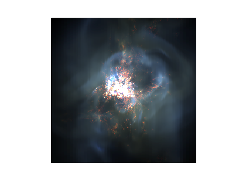
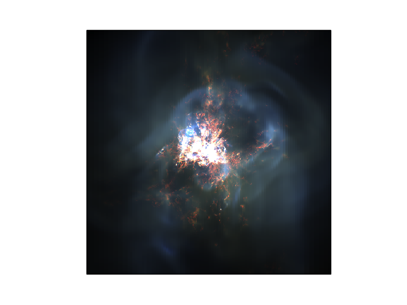
Synthetic X-ray composite image in 0.3-1.2 (red), 1.2-2 (green) and 2-7 keV (blue) bands. This is showing the central 100 kpc region of a simulated galaxy cluster under the influence of supermassive black hole feedback. The observational angle is randomly chosen to be 23 degrees from the z-axis in the y-z plane. Each individual channel has been rescaled to bring out fainter features. The “bubbles” seen in the simulations are created by shock waves and the enhanced soft X-ray (red) traces the cold clumps and filaments that condensed out of the diffuse intracluster medium.

Description:

Early X-ray observations indicate that many galaxy clusters possess a cool core where the intracluster medium has a high density and low temperature, with a radiative cooling time much shorter than the Hubble time. In the absence of any heating source, these cool-core clusters are expected to develop cooling flows of hundred to a thousand solar masses per year in a steady state. However, recent observations by Chandra and XMM-Newton have revealed a deficit of cooler X-ray gas at temperatures below 1/3 of the viral temperature. The observed star formation rate is also typically much lower than the classical rate. This discrepancy is referred to as the “cooling flow problem”. The absence of a classical cooling flow indicates that radiative cooling is suppressed by some heating mechanism.

It is now widely accepted that AGN feedback is the major heating source in the center of most, if not all, cool-core clusters, and that it offers the most promising solution to the classic “cooling flow problem.” Many cool-core clusters also harbor line emitting cold gas, which sometimes exists in filamentary structures with a spatial extent of up to a few tens of kpc. Some filaments host star forming clumps, and many filaments specially correspond to soft X-ray features and dust lanes, indicating that the gas is multiphase.

We perform adaptive mesh hydrodynamic simulations using Enzo to study the effect of momentum-driven AGN feedback powered by the accretion of cold gas onto the supermassive black hole in the center of the cluster. As the figure shows, AGN jets produce shock waves (seen in the hard X-ray band in blue) that heat up the diffuse intracluster medium, but also locally drive non-linear instabilities that cause hot gas to cool into cold filaments (seen in the soft X-ray band in red). This figure is to be comparable to the famous Chandra X-ray map of the Perseus cluster.

The simulation data is analyzed with the help of the yt package. This figure is used in our paper published in the Astrophysical Journal.

Products

• PDF

Source

import matplotlib
matplotlib.use('Agg')
from yt.mods import *
from yt.config import ytcfg; ytcfg["yt","serialize"] = "False"
import numpy as numpy
import matplotlib.pylab as pylab

def X_composite(i=50,widthkpc=100,thicknesskpc=5000,theta=0.9,scale=[0.1,1.0,1.0], N=512):
 import yt.analysis_modules.spectral_integrator.spectral_frequency_integrator as SI
 SI.add_xray_emissivity_field(0.3,1.2,with_metals=False,constant_metallicity=0.5)   #red
 SI.add_xray_emissivity_field(1.2,2.0,with_metals=False,constant_metallicity=0.5)   #green
 SI.add_xray_emissivity_field(2.0,7.0,with_metals=False,constant_metallicity=0.5)   #blue
 fn = name_pattern %(i,i)
 pf = load(fn)
 center=[0.5,0.5,0.5]
 thickness = thicknesskpc/pf['kpc']
 width=widthkpc/pf['kpc']
 L = [0,numpy.sin(theta), numpy.cos(theta)]
 R = off_axis_projection(pf, center, L, (width,width,thickness), N, "Xray_Emissivity_0.3_1.2keV")
 G = off_axis_projection(pf, center, L, (width,width,thickness), N, "Xray_Emissivity_1.2_2.0keV")
 B = off_axis_projection(pf, center, L, (width,width,thickness), N, "Xray_Emissivity_2.0_7.0keV")
 write_projection(R, "%s_offaxis_projection%.1f_Xray_R.png" % (pf, theta), colorbar_label="X ray Surface Brightness "+r"($ergs \, s^{-1} \, cm^{-2}$)")
 write_projection(G, "%s_offaxis_projection%.1f_Xray_G.png" % (pf, theta), colorbar_label="X ray Surface Brightness "+r"($ergs \, s^{-1} \, cm^{-2}$)")
 write_projection(B, "%s_offaxis_projection%.1f_Xray_B.png" % (pf, theta), colorbar_label="X ray Surface Brightness "+r"($ergs \, s^{-1} \, cm^{-2}$)")
 im_r=numpy.zeros((R.shape[0],R.shape[1],3),'uint8')
 im_g=numpy.zeros_like(im_r)
 im_b=numpy.zeros_like(im_r)
 RGB=numpy.zeros_like(im_r)
 high=R>scale[0]*numpy.max(R)   ##rescale R
 R[high]=scale[0]*numpy.max(R)
 high=G>scale[1]*numpy.max(G)   ##rescale R
 G[high]=scale[1]*numpy.max(G)
 high=B>scale[2]*numpy.max(B)   ##rescale R
 B[high]=scale[2]*numpy.max(B)
 im_r[:,:,0]=255.9*(R-numpy.min(R))/(numpy.max(R)-numpy.min(R))
 im_g[:,:,1]=255.9*(G-numpy.min(G))/(numpy.max(G)-numpy.min(G))
 im_b[:,:,2]=255.9*(B-numpy.min(B))/(numpy.max(B)-numpy.min(B))
 RGB[:,:,0]=255.9*(R-numpy.min(R))/(numpy.max(R)-numpy.min(R))
 RGB[:,:,1]=255.9*(G-numpy.min(G))/(numpy.max(G)-numpy.min(G))
 RGB[:,:,2]=255.9*(B-numpy.min(B))/(numpy.max(B)-numpy.min(B))
 stest = 'stest_%04i' %i
 pylab.figure(3)
 pylab.imshow(im_b,origin="lower", interpolation="nearest")
 pylab.savefig("im_b.png")
 pylab.figure(4)
 pylab.imshow(im_g,origin="lower", interpolation="nearest")
 pylab.savefig("im_g.png")
 pylab.figure(5)
 pylab.imshow(im_r,origin="lower", interpolation="nearest")
 pylab.savefig("im_r.png")
 pylab.figure(1)
 pylab.imshow(RGB,origin="lower", interpolation="nearest")
 pylab.tick_params(axis='both',which='both',bottom='off',top='off',left='off',right='off',labelbottom='off',labelleft='off',labelright='off')
 pylab.savefig(stest+"X_composite.png")
 return