Entry 21
Authors
- Bill Baxter
Products
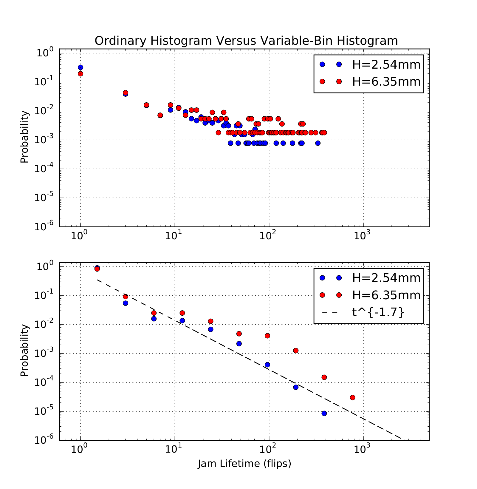
Power-law behavior \(P (x) = Ax^{−b}\) is commonly found in a wide variety of experimental data. The case where \(b > 0\) so that \(P(x)\) becomes rapidly smaller with increasing \(x\) is especially common. The example shown here is from a laboratory experiment on the formation of jams (static plugs of grains which are supported by the walls) in a granular material falling under gravity through a featureless vertical channel. Our measure of time is the number of instances in which the vertical channel is flipped upside down to allow the grains to fall. Most of the time, all the grains fall and no jams form. The probability of a jam forming is very low; however, once a jam forms it may last for quite some time. The data here show, for two different grain sizes, the probability that, once a jam forms, that jam will survive for a certain number of flips of the channel.
In the top figure, we employ Matplotlib [1] and a simple histogram with all bins being the same size. Note the data which fall along horizontal lines. These correspond to bins with only one, two, or three events. Most bins have no events at all and have been filtered from the data. On a log-log plot, a power-law would appear as a straight line. Clearly more data is needed to be able to see trends at higher jam lifetimes. But this is problematic in this experiment as jams occur very seldom and long-lasting jams are extremely rare. The experiment might have to run for years to generate sufficient data.
The better solution is shown in the bottom figure which uses a histogram with variable bin sizes. Here, the bin size gets larger as the jam lifetime gets longer [2]; each bin is twice as wide as the bin that preceeds it. The result is fewer bins with more counts in each and a bin spacing that is uniform on a log-log plot. Each bin’s count is normalized by the bin width. The resulting data is much cleaner and extends for more decades. The line representing a power-law with exponent 1.7 is simply to guide the eye.
References
[1] J. D. Hunter. Matplotlib: A 2d graphics environment. Computing In Science & Engineering, 9(3):90–95, 2007.
[2] Padraig Mac Carron and Ralph Kenna. Universal properties of mythological networks. European Physics Letters, 99:28002, 2012.
Source
#Illustrates advantage of variable-bin histograms for data with a power law
#behavior.  The tail of the power law will be clear and easier to interpret.
#
#  Bill Baxter,   gwb6@psu.edu,  Penn State Erie, The Behrend College
#      Original Data.   04/13/2015
#
import numpy as np
import matplotlib.pyplot as plt

h100=np.loadtxt(file("h0.100.lengths"))
h250=np.loadtxt(file("h0.250.lengths"))

bins2b=np.arange(0,401,2)
x2=np.arange(1,401,2)

H100,x=np.histogram(h100,bins2b,normed=True)
H250,x=np.histogram(h250,bins2b,normed=True)

plt.subplots_adjust(wspace=0.5)
plt.subplot(211)

plt.loglog(x2[H100>0],H100[H100>0],'bo')
plt.loglog(x2[H250>0],H250[H250>0],'ro')
plt.legend((r'H=2.54mm', r'H=6.35mm'))
plt.xlim(0.6,5000.)
plt.ylim(1E-6,1.4)
plt.ylabel("Probability")
plt.title("Ordinary Histogram Versus Variable-Bin Histogram")
plt.grid(color='k',which='major')


plt.subplot(212)
bins_ln=np.arange(0,14,1)
width_ln=np.arange(0,14,1)
x2=np.arange(0.,14.,1.)
xmin=1.
plt.grid(color='k',)
a=2
for i in np.arange(1,15,1):
    xleft=xmin*a**(i-1)
    xright=xmin*a**i
    range=xright-xleft
    bins_ln[i-1]=xleft
    width_ln[i-1]=range
    print xleft,"  ",xright,"   ",range

H100,x=np.histogram(h100,bins_ln)
H250,x=np.histogram(h250,bins_ln)

Hist100=np.arange(0.,13.,1.)
Hist250=np.arange(0.,13.,1.)

#Normalize each bin value by the new binwidth.
for i in np.arange(0,13,1):
    Hist100[i]=float(H100[i])/float(width_ln[i])
    Hist250[i]=float(H250[i])/float(width_ln[i])
    x2[i]=float(bins_ln[i])+float(width_ln[i])/2.

#Normalize so we plot PROBABILITIES rather than COUNTS
Hist100_sum=Hist100.sum()
Hist250_sum=Hist250.sum()
Hist100=Hist100/Hist100_sum
Hist250=Hist250/Hist250_sum

#Create a power law line to guide the eye.
f=np.zeros(14 )
i=0
while i<14 :
#    f[i]=0.3/(x2[i]**1.5)
    f[i]=0.7/(x2[i]**1.7)
    i=i+1

plt.loglog(x2[Hist100>0],Hist100[Hist100>0],'bo')
plt.loglog(x2[Hist250>0],Hist250[Hist250>0],'ro')
plt.loglog(x2,f,'k--')
plt.legend((r'H=2.54mm', r'H=6.35mm', r't^{-1.7}'))
plt.grid(color='k',which='major')
plt.xlabel("Jam Lifetime (flips)")
plt.ylabel("Probability")
plt.xlim(0.6,5000.)
plt.ylim(1E-6,1.4)

plt.show()