Entry 4
Authors
- Jovan Veljanoski
Galaxy formation and evolution are ones of the fundamental processes in astrophysics that are not fully understood. According to the currently preferred cosmological model, galaxies are at least partly built in a hierarchical manner via the accretion of smaller fragments or dwarf galaxies. The evidence of these processes is best visible in the haloes (outskirts) of galaxies, where the accreted dwarf galaxies are tidally disrupted and form stellar streams. By studying these accreted components we can infer key properties of the host galaxy, such as its gravitation potential and assembly history.
Studying of galaxy haloes is a formidable observational challenge, because the density of stars in these regions is low, making them difficult to observe. An alternative approach is to use globular clusters (GCs) as tracers of the stellar properties. GCs are spherical collections of stars, comprising several thousand to several million members in each, making them very bright and easily observable objects. Due to its close proximity, our nearest neighbour, the Andromeda galaxy (M31) is a desirable target. It hosts more than 500 confirmed GCs, listed in the Revised Bologna Catalogue (RBC), over 100 of which are located in the far outskirts of the galaxy. In the past several years I led a major spectroscopic campaign, aiming to determine the radial velocities of the halo GCs around M31. The plot I am presenting conveys the key results coming from this work.
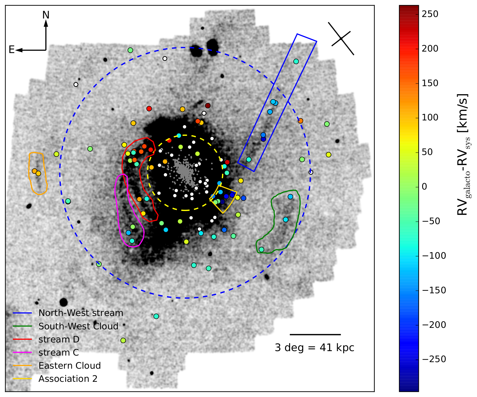
The basis of the plot is a panoramic view of the metal poor stars in M31. The map is slightly smoothed to enhance the various stellar over-densities in the halo, marked with the coloured contours, which are the remnants of past accretion events. The coloured points represent the GCs in the halo of M31, which were part of the spectroscopic survey. The colours represent their radial velocities, as if they were observed from the centre of our Galaxy, and they are corrected for the systemic motion of M31. The white points are halo GCs that are not yet spectroscopically observed, while the gray points are GCs lying in the disk of M31. The schematic on the top right of the plot corresponds to the orientation of the major and minor axis of M31. To guide the two circles having radii of 30 and 130 kpc are placed.
The first key result it is that the GCs in the halo are primarily projecting onto the substructures. Moreover, the groups GCs lying along particular substructures exhibit various velocity patterns and correlations, linking them to the stellar streams. Thus, it is seen how we can use GCs to study the build up of galaxies. The second key point is the detection of a coherent rotation of the halo GC system of M31. Looking at the map, one can notice that the GCs in the top left region have systematically higher velocities than those in the bottom right. This has important implications regarding galaxy formation models.
This work and plot are published in: Veljanoski et al., 2014, MNRAS, 442, 2929 Link
Source
'''
Fancy map creator : creates the map M31, adds the halo GCs, color-coded
according to their velocities. The inner GCs are also marked with grey points.
To guide the eye, rings having radii of 30 and 130 kpc are also displayed.

In addition, regions of particular interest are also labelled.
'''
# import pywcs
import pylab as p
from scipy import *
from readcol import readcol
import astropy.wcs as pywcs
import astropy.io.fits as pf
from matplotlib.patches import Circle
from scipy.ndimage.filters import gaussian_filter

##M31 data
ra_m31 = 0.18648115831219983    # in radians
dec_m31 = 0.72028283794580406   # in radians
ra_m31_deg = rad2deg(ra_m31)
dec_m31_deg = rad2deg(dec_m31)
gal_vel_m31 = -109.260841724    # km/s


##reading the raw map
themap = pf.open('m31map/m31Map.fits')
map = themap[0].data
#Smoothing the background map
smap = gaussian_filter(map,2.2,0)

## Reading the data catalogue
input = readcol('catalogues/fullM31velocitycatalogue4.5.2', twod = True)
ra         = (input[:,1]).astype(float)
dec        = (input[:,2]).astype(float)
gal_vel    = (input[:,9]).astype(float)
projectedR = (input[:,8]).astype(float)
ID         = input[:,0]
notes      = input[:,11]
gctype     = input[:,14]
src        = input[:,12]

# reading the positions of the clusters which were not observed spectroscopically
p_obs       = readcol('catalogues/PAndAS_position_obs', twod = True)
p_obs_ra    = (p_obs[:,1]).astype(float)
p_obs_dec   = (p_obs[:,2]).astype(float)
p_obs_rproj = (p_obs[:,6]).astype(float)
p_obs_obs   = p_obs[:,7]

## Reading substruction regions
ass2reg  = readcol('regions/G1_overdensity2.wcs',twod = False)
strDreg  = readcol('regions/stream_D.wcs2',twod       = False)
strCreg  = readcol('regions/streamC.reg',twod         = False)
strNWreg = readcol('regions/NWS.reg',twod             = False)
strSWreg = readcol('regions/SW_stream.wcs',twod       = False)
strESreg = readcol('regions/EasternShell.wcs',twod    = False)


## Cluster selection
# Select clusters that will apear on the map, color coded by their velocity
ind = (projectedR > 30.0) | (src == 'mine')
# this selects the clusters from PAndAS that were not observed spectroscopically
obs_ind = (p_obs_rproj >=10) & (p_obs_obs == 'No')
# these are the clusters from the RBC
ind_rbc = src == 'RBC'

#To simplify selection of subsystems, lets make these selection indices
ra_ind      = ra[ind]
dec_ind     = dec[ind]
gal_vel_ind = gal_vel[ind] - gal_vel_m31
# same for the un-observed PAndAS clusters
ra_obs_ind  = p_obs_ra[obs_ind]
dec_obs_ind = p_obs_dec[obs_ind]
# the positions for the RBC clusters, for convenience
ra_rbc      = ra[ind_rbc]
dec_rbc     = dec[ind_rbc]
ID_rbc = ID[ind_rbc]


## Converting coordinates
# Converting coordinates from ra/dec to pixel coordinates so they can be
# overplotted on the M31 map
# reading in the map WCS
pywcsObject = pywcs.WCS(themap[0].header)
# for general plotting of GC, labels etc..
x_pix,y_pix = pywcsObject.wcs_world2pix([ra[ind]],[dec[ind]],0)
# for the velocity colour plot
x_pix_cmap,y_pix_cmap = pywcsObject.wcs_world2pix([ra_ind],[dec_ind],0)
# for the center of M31, for the circles on the plot
x_pix_m31,y_pix_m31 = pywcsObject.wcs_world2pix([ra_m31_deg],[dec_m31_deg],0)
#converting the regions, so they can appear on the map
x_ass2reg,y_ass2reg = pywcsObject.wcs_world2pix([ass2reg[0]],[ass2reg[1]],0)
x_strDreg,y_strDreg = pywcsObject.wcs_world2pix([strDreg[0]],[strDreg[1]],0)
x_strCreg,y_strCreg = pywcsObject.wcs_world2pix([strCreg[0]],[strCreg[1]],0)
x_strNWreg,y_strNWreg = pywcsObject.wcs_world2pix([strNWreg[0]],[strNWreg[1]],0)
x_strSWreg,y_strSWreg = pywcsObject.wcs_world2pix([strSWreg[0]],[strSWreg[1]],0)
x_strESreg,y_strESreg = pywcsObject.wcs_world2pix([strESreg[0]],[strESreg[1]],0)
# for the clusters not spectroscopically observed
x_p_obs, y_p_obs = pywcsObject.wcs_world2pix([ra_obs_ind],[dec_obs_ind],0)
# for the RBC clusters
x_rbc, y_rbc = pywcsObject.wcs_world2pix([ra_rbc],[dec_rbc],0)

## Creating the colour mapped moints
points = zip(x_pix_cmap,y_pix_cmap)
points3 = sorted(zip(gal_vel_ind,points))

for i,pp in enumerate(points3):
    gal_vel_ind[i] = pp[0]
    x_pix_cmap[i] = pp[1][0]
    y_pix_cmap[i] = pp[1][1]


## Master Plot
p.figure(figsize=(12, 9), dpi=300, facecolor='w', edgecolor='k')

# plotting the map and the GCs
# the M31 maps, smoothed
p.imshow(smap,
         vmin=1,
         vmax=121,
         origin='lower',
         cmap='binary')
# The GCs coming from the RBC, in the inner regions of M31.
p.scatter(x_rbc,y_rbc,
          color = 'gray',
          s=5,
          edgecolor='none',
          lw=0.3)
# the GCs in the halo without velocities
p.scatter(x_p_obs,y_p_obs,
          color = 'white',
          s=30,
          edgecolor='black',
          lw=1)
# The GCs with velocities in the halo
p.scatter(x_pix_cmap,y_pix_cmap,
          c=gal_vel_ind,
          s=45,
          edgecolor='black',
          lw=0.7)

 # makes the colorbar appear, with the ticks at the right places
p.colorbar(ticks = range(-250,300,50))
ax  = p.gca() # axis parameters modifier
fig = p.gcf() # figures parameters modifier

# rendering the x/y axis invisible
ax.yaxis.set_visible(False)
ax.xaxis.set_visible(False)

# setting the axis limits;
# in this case this selects which portion of the map will be displayed
p.ylim([130,1465]) # set limits on y axis
p.xlim([270,1545]) # set limits on x axis

# Adding raw text on the plot
# label1 is the right hand side axis label
label1 = p.text(1830, 1131,
                r'RV$_{\rm galacto}$-RV$_{\rm sys}$ [km/s]',
                rotation = 'vertical',
                fontsize = 17)
# label2 is the text showing scale of the plot
label2 = p.text(1200, 270,
                '3 deg = 41 kpc',
                rotation = 'horizontal',
                fontsize = 14)
#line showing the scale of the plot
p.plot([1255,1427],[327,327],lw = 1.7,color = 'black')

# Adding circles, marking 30 and 130 kpc radii, to guide the eye
# the 30 kpc circle
rad30 = Circle((x_pix_m31,y_pix_m31),
               radius =130,
               facecolor = 'none',
               edgecolor = 'yellow',
               lw = 1.7)
# settin up additional parameters for the circle, the linestyle
p.setp(rad30, ls='dashed')
# adding the circle to the plot
fig.gca().add_artist(rad30)
#the 130 kpc circle
rad130 = Circle((x_pix_m31,y_pix_m31),
                radius =433,
                facecolor = 'none',
                edgecolor = 'blue',
                lw = 1.7)
# settin up additional parameters for the circle, the linestyle
p.setp(rad130, ls='dashed')
# adding the circle to the plot
fig.gca().add_artist(rad130)

# Adding the compass on the plot
# arrow pointing north
p.arrow(410,1310,0,100,
        lw=1.5,
        fill=True,
        length_includes_head=True,
        head_length=17,
        head_width= 10,
        color = 'black')
# arrow pointing east
p.arrow(410,1310,-100,0,
        lw=1.5,
        fill=True,
        length_includes_head=True,
        head_length=17,
        head_width= 10,
        color = 'black')
# label for North, 'N'
p.text(397,1420,'N',fontsize = 14)
# label for East, 'E'
p.text(280,1300,'E',fontsize = 14)

# Adding major/minor axis schematic to the plot
#major axis
p.scatter([1430],[1350], s = 7)
p.plot([1430,1430+70*sin(deg2rad(-38))],
       [1350,1350+70*cos(deg2rad(-38))],
       lw = 1.5,
       color = 'black')
p.plot([1430,1430+70*sin(deg2rad(-38+180))],
       [1350,1350+70*cos(deg2rad(-38+180))],
       lw = 1.5,
       color = 'black')
#minor axis
p.plot([1430,1430+0.56*70*sin(deg2rad(-38+90))],
       [1350,1350+0.56*70*cos(deg2rad(-38+90))],
       lw = 1.5,
       color = 'black')
p.plot([1430,1430+0.56*70*sin(deg2rad(-38-90))],
       [1350,1350+0.56*70*cos(deg2rad(-38-90))],
       lw = 1.5,
       color = 'black')


# # Adding the regions, cold substructures to the map
p.plot(x_strNWreg[0], y_strNWreg[0],
       color = 'blue',
       lw = 1.5,
       label = 'North-West stream')
p.plot(x_strSWreg[0], y_strSWreg[0],
       color = 'green',
       lw = 1.5,
       label = 'South-West Cloud')
p.plot(x_strDreg[0],  y_strDreg[0],
       color = 'red',
       lw = 1.5,
       label = 'stream D')
p.plot(x_strCreg[0],  y_strCreg[0],
       color = 'magenta',
       lw = 1.5,
       label = 'stream C')
p.plot(x_strESreg[0], y_strESreg[0],
       color = 'orange',
       lw = 1.5,
       label = 'Eastern Cloud')
p.plot(x_ass2reg[0],  y_ass2reg[0],
       color = 'gold',
       lw = 1.5,
       label = 'Association 2')

# the legend..
p.rc('legend',**{'fontsize':12})
p.legend(scatterpoints=1,numpoints=1,loc = 3, frameon=False)


# Saving the plot to disk
p.savefig('bigmap.pdf',
          dpi=300,
          orientation='landscape',
          bbox_inches = 'tight',
          bbox_extra_artists=[label1])


# End of File