Entry 6
Authors
- Vicky Scowcroft
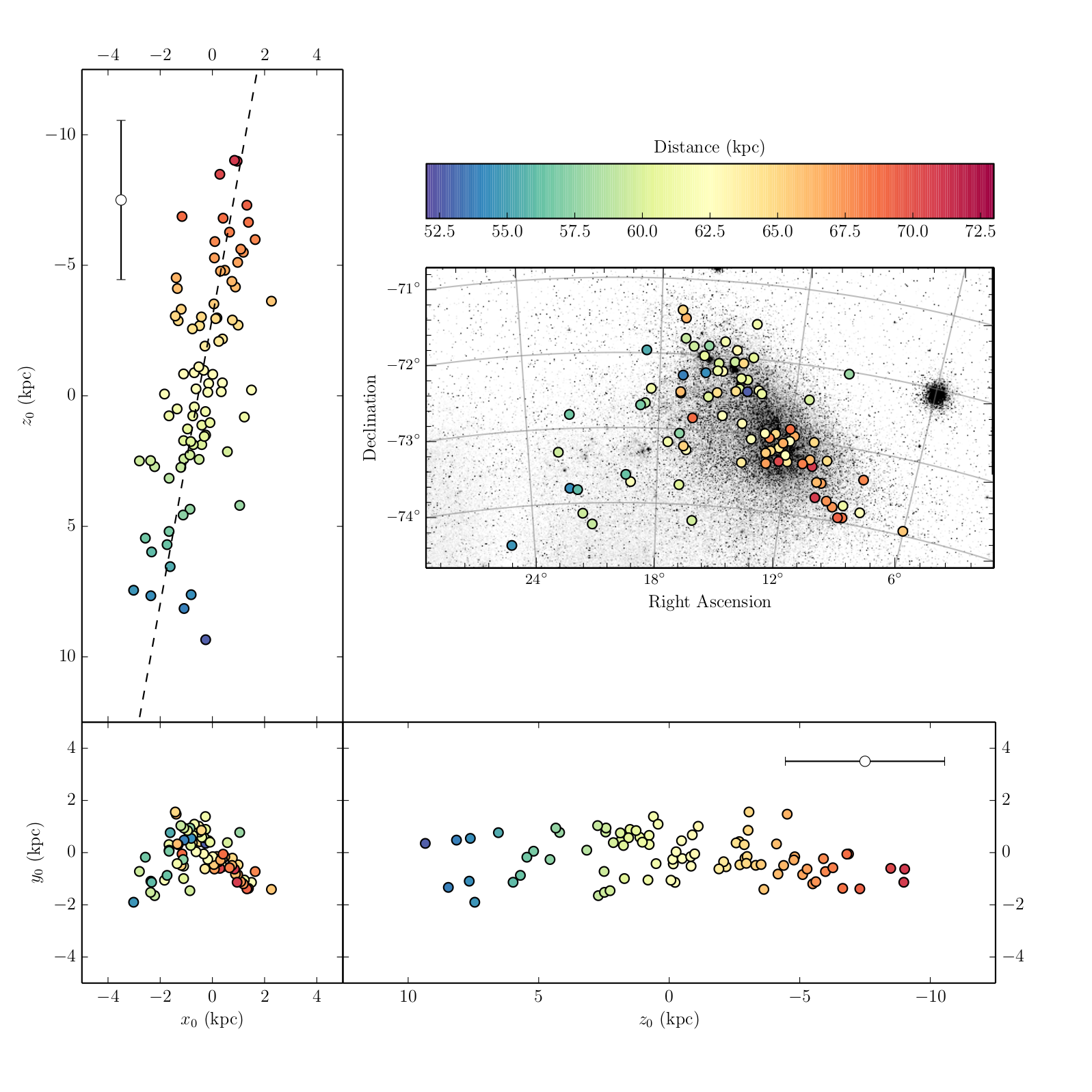
The 3-dimensional structure of the Small Magellanic Cloud as revealed by Cepheids
This plot shows the 3-dimensional positions of Cepheids (a type of variable star) in the Small Magellanic Cloud (SMC) galaxy. The distances to each Cepheid were measured using mid-infrared observations from the Spitzer space telescope.
The top right panel shows the stars in Celestial coordinates, color coded by their distance from Earth, plotted on top of a digital sky survey image of the SMC. This panel shows how the galaxy and its Cepheids appear to us from Earth. The Cepheids are color-coded according to their distance from Earth. Those closer to us are shown in blue, those further away are shown in red.
The bottom left panel shows these same stars now projected into a cartesian coordinate system. The color coding is the same as the initial plot. The x0-y0 projection is essentially the same as the Celestial projection. Note the size of this panel — the cartesian panels are all plotted on the same scale, so the fact that the galaxy appears small in this panel is because it appears small to us on the sky.
The top left and bottom right panels are plotted to the same scale as the bottom left panel, and are significantly extended along the z0 axis. This axis shows the distance between us and the individual Cepheids. We are now seeing the true 3-dimensional structure of the SMC. It is dramatically elongated along the line of sight, and is tilted such that the North Eastern side is approximately 20 kpc closer than the South Western side.
This plot originally appeared in “The Carnegie Hubble Program: The Distance and Structure of the SMC as Revealed by Mid–infrared Observations of Cepheids”, Scowcroft et al. (2015), arXiv:1502.06995, ApJ in press.
Source
#!/usr/bin/env/python

## Program to plot the Cepheids distances as a fn of position

import numpy as np
import matplotlib.pyplot as mp
import glob
import re
import os
from scipy.optimize import curve_fit
import coordinate_conversion as cc
from matplotlib import cm
from scipy.interpolate import griddata
import numpy.ma as ma
import matplotlib.gridspec as gridspec
import aplpy


from mpl_toolkits.mplot3d import Axes3D


os.environ['PATH'] = os.environ['PATH'] + ':/usr/texbin'
matplotlib.rc('text',usetex=True)
from matplotlib import rcParams
rcParams['font.family'] = 'serif'
rcParams['font.serif'] = ['Garamond']


band = []
period = []
mag = []
err = []
cepid = []
ra = []
dec = []
cepname = []
ra_arr = []
dec_arr = []
logp = []
distmod = []
disterr = []
distance = []
distmoderr = []

## Coordintes of SMC centre
## A = 00:52:44.8
## D = -72:49:43

A, D = cc.todeg("00:52:44.8", "-72:49:43")

#print A, D

Arad = A * np.pi / 180.
Drad = D * np.pi / 180.


distmod_high = 0
distmod_low = 100
for cep in open("dereddened_smc_cepheid_data","r"):
	data = cep.split()
	logp.append(data[1])
	#Cutting data on log period
	if ((float(data[1]) > 0.77815125038364363) & (float(data[1]) < 1.77815125038364363)):
		cepid.append(data[0])

		ra = data[2]+":"+data[3]+":"+data[4]
		dec = data[5]+":"+data[6]+":"+data[7]

		radeg, decdeg = cc.todeg(ra,dec)
		rarad = radeg * np.pi / 180.
		decrad = decdeg * np.pi / 180.
		ra_arr.append(radeg)
		dec_arr.append(decdeg)


		distmod.append(float(data[8]))
		distmoderr.append(float(data[9]))
		if distmod > distmod_high:
			distmod_high = distmod
		if distmod < distmod_low:
			distmod_low = distmod

		tempdist = 10**((float(data[8]) + 5.)/5.) / 1000.
		distance.append(tempdist)
		tempdisterr = 0.461*tempdist*sqrt(float(data[9])**2 + 0.108**2)
		disterr.append(tempdisterr)


distance = np.array(distance)
logp = np.array(logp)
cepid = np.array(cepid)
ra_arr = np.array(ra_arr)
dec_arr = np.array(dec_arr)
disterr = np.array(disterr)
rarad = ra_arr * np.pi / 180.
decrad = dec_arr * np.pi / 180.

mp.clf()
ra0, dec0 = cc.todeg("00:52:44.8", "-72:49:43")
Rsmc = 61.94


ra0rad = ra0 * np.pi / 180.
dec0rad = dec0 * np.pi / 180.

## Conversion to cartesian coordinate system

x0 = - distance * cos(decrad) * sin (rarad - ra0rad)
y0 = (distance * sin(decrad) * cos(dec0rad)) - (distance * cos(decrad) * sin(dec0rad) * cos(rarad - ra0rad))
z0 = Rsmc - (distance * cos(decrad) * cos(dec0rad) * cos(rarad - ra0rad)) - (distance * sin(decrad) * sin(dec0rad))

def tilt(distance,  slope, zp):
	return( slope * distance + zp)

popt, pcov = curve_fit(tilt,  z0, x0)


slope = popt[0]
zp = popt[1]
eslope = pcov[0][0]
ezp = pcov[1][1]
#print "Tilt = ", slope, "+-", eslope


mp.close()
fig = mp.figure(figsize=(10,10))


## Bottom left

axp1 = fig.add_axes([0.075, 0.1, 0.2389, 0.2389])
axp1.axis([-5,5, -5, 5])
im = axp1.scatter(x0, y0, c=distance, cmap=cm.Spectral_r, s=40, vmin=52.,vmax =73.)
xlabel('$x_0$ (kpc)')
ylabel('$y_0$ (kpc)')


## Top left
axp2 = fig.add_axes([0.075, 0.3389, 0.2389, 0.5975])

axp2.axis([-5,5, 12.5, -12.5])
axp2.errorbar(-3.5, -7.5, yerr = 3.05,ls='None',c='k')
axp2.plot(-3.5, -7.5, "wo", ms=7)
axp2.scatter(x0, z0, s=40,  c=distance, cmap=cm.Spectral_r, vmin=52., vmax=73.)
axp2.xaxis.set_tick_params(labeltop='on')
axp2.xaxis.set_tick_params(labelbottom='off')
y = np.arange(-15, 15, 0.01)
x = slope* y + zp
axp2.plot(x, y, "k--")
ylabel('$z_0$ (kpc)')

## Bottom right
axp3 = fig.add_axes([0.3139, 0.1, 0.5975, 0.2389])
axp3.axis([12.5, -12.5, -5, 5])
axp3.scatter(z0, y0, c=distance, cmap=cm.Spectral_r,s=40, vmin=52., vmax = 73.)
axp3.errorbar(-7.5, 3.5, xerr = 3.05,ls='None',c='k')
axp3.plot(-7.5, 3.5, "wo", ms=7)
xlabel('$z_0$ (kpc)')
axp3.yaxis.set_tick_params(labelright='on')
axp3.yaxis.set_tick_params(labelleft='off')

## Top right

big_image = "smc_dss_huge.fits"
small_image = "smc_dss.fits"
big_smc = aplpy.FITSFigure(big_image,north='True', figure = fig, subplot=[0.39, 0.48, 0.52, 0.275])
big_smc.set_theme('publication')

big_smc.add_grid()
big_smc.grid.set_color('grey')
big_smc.grid.show()

big_smc.show_grayscale(vmin=12000,vmax=16500,invert='true')
big_smc.recenter(A+2.5, D, radius=2.0)

big_smc.tick_labels.set_font(size='small')
big_smc.tick_labels.set_xformat("dd")
big_smc.tick_labels.set_yformat("dd")
big_smc.show_markers(ra_arr,dec_arr, c=distance, cmap=cm.Spectral_r, s=40, vmin=52., vmax = 73., zorder=4)


xlabel('Right Ascension')
ylabel('Declination')


cbar_ax = fig.add_axes([0.39, 0.8, 0.52, 0.05])
cb = fig.colorbar(im, cax=cbar_ax, orientation='horizontal')
im.set_clim(52.,73.)
cb.set_label("Distance (kpc)", labelpad=-68)
mp.show()

mp.savefig("scowcroft_plotting_contest.pdf", transparent="True")


mp.show()