Entry 9

Authors

• Suoqing Ji
• Robert Fisher

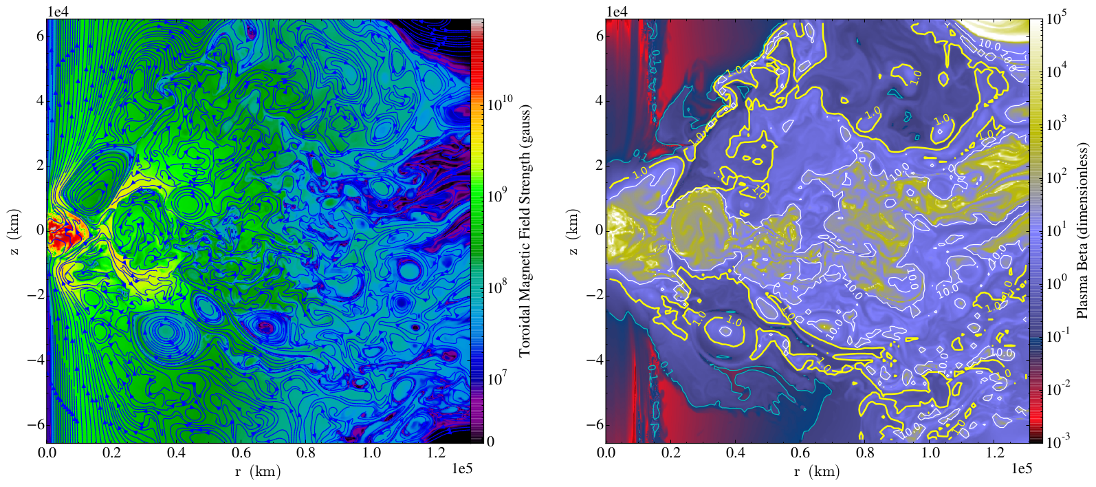
Visualization of Magnetized Binary White Dwarf Merger

Type Ia supernovae (SNe Ia) result from the thermonuclear explosion of a carbon-oxygen white dwarf star. The brightnesses of typical Type Ia supernovae explosions are highly similar, providing us with a standard candle with which we can accurately measure space and time in the cosmos. Using Type Ia supernovae, astronomers have accurately measured the rate at which space itself is expanding, and have inferred the existence of a mysterious new type of energy – dark energy. However, the nature of the progenitors which give rise to Type Ia supernovae, and of the explosion mechanism itself, remain poorly understood.

One possible way to give rise to Type Ia supernovae is the merging of white dwarf binaries, where the merging white binary system produces a rapidly-spinning white dwarf merger surrounded by a hot disk. The differentially-rotating disk is highly-unstable to an initially weak magnetic field, which is significantly amplified as fluid elements are destabilized by the Lorentz force, referred to as the magnetorotational instability (MRI).

We perform the first multidimensional simulations of these white dwarf merger remnants to include a full treatment of magnetohydrodynamics, and demonstrate, for the first time, that MRI produces a high-field magnetic white dwarf, with a surface field exceeding \(10^8\) gauss.

The visualization of the simulation data is produced using Python matplotlib and yt (http://yt-project.org) packages. The two frames are plotted on \(r-z\) plane in 2-D axisymmetric cylindrical coordinates.

The left frame shows the structure of magnetic field, with lines of poloidal magnetic field in the \(r-z\) plane superposed against a color raster plot of the toroidal magnetic field \(B_\phi\). The field structure is highly turbulent and disordered due to MRI, with loops of heated magnetic flux rising buoyantly above the accretion disk, and bi-conical jets carrying open field lines away from the merger.

The right frame shows the plasma \(\beta\) value, which is the ratio of gas pressure to magnetic pressure, with contours of \(\beta = 0.1, 1, 10\) superposed. Regions of high \(\beta\) are dominated by gas pressure, while those with low \(\beta\) are supported by magnetic pressure. The merger and accretion disk themselves remain relatively weakly-magnetized (\(\beta \gg 1\)). The disk corona is magnetically important (\(\beta \sim 1\)), whereas the bi-conical jets are strongly-magnetized (\(\beta \ll 1\)).

Movies of the simulations are available here.

Products

• PDF

Source

import yt
import numpy as np
import matplotlib.pyplot as plt
from mpl_toolkits.axes_grid1 import AxesGrid

@yt.derived_field(name="toroidal_magnetic_field_strength",
                  units="sqrt(g / cm) / s")
def _toroida_magnetic_field_strength(field,data):
    return np.abs(data["magnetic_field_z"])

def _get_fig(field):
    ds = yt.load("sub2D_hdf5_chk_1000")
    slc = yt.SlicePlot(ds, "theta", field, origin="center-left-window")

    if field == "toroidal_magnetic_field_strength":
        slc.set_cmap(field, "spectral")
        slc.set_log(field, True, linthresh=1.e7)
        slc.set_colorbar_label(field, "Toroidal Magnetic Field Strength (gauss)")
        slc.annotate_streamlines("magnetic_field_x", "magnetic_field_y",
                                                    factor=2., density=6.)
    elif field == "plasma_beta":
    	slc.set_cmap(field, "gist_stern")
    	slc.set_zlim(field, 1.e-3, 1.e5)
        slc.set_colorbar_label(field, "Plasma Beta (dimensionless)")
        slc.annotate_contour(field,
                             ncont=1,
                             factor=7.,
                             take_log=False,
                             clim=(1.e0,1.e0),
                             label=True, 
                             plot_args={"colors": "yellow", "linewidths": 2},
                             text_args={"fmt": "%1.1f"})
        slc.annotate_contour(field,
                             ncont=2,
                             factor=7.,
                             take_log=False,
                             clim=(1.e-1,1.e1),
                             label=True, 
        	                 plot_args={"colors": ("c","w"), "linewidths": 1},
                             text_args={"fmt": "%1.1f"})

    return slc

fig = plt.figure()

grid = AxesGrid(fig, (0., 0., 1.5, 1.5),
                nrows_ncols=(1, 2),
                axes_pad=2.,
                label_mode="all",
                share_all=False,
                cbar_location="right",
                cbar_mode="each",
                cbar_size="3%",
                cbar_pad="0%")

fields = ["toroidal_magnetic_field_strength", "plasma_beta"]

for i, field in enumerate(fields):
    slc = _get_fig(field)
    plot = slc.plots[field]
    plot.figure = fig
    plot.axes = grid[i].axes
    plot.cax = grid.cbar_axes[i]
    slc._setup_plots()
    slc.run_callbacks()

fig.savefig("magnetic_white_dwarf_merger.pdf", bbox_inches = "tight")

• sub2D_hdf5_chk_1000.hdf