In order to calculate ionic abundances in a real nebula, it is necessary to
know the electron temperature and density where the various ionic emissions
are produced. In some physical contexts it makes sense to view the structure
of a nebula as an ``onion skin,'' where the ionization drops off radially
from some central source of ionizing radiation, and T drops somewhat while N
Two tasks in the nebular package were designed to model nebulae in just
this way, with separate zones of low-, intermediate-, and high-ionization.
The nebular physical parameters are derived within each zone by making
simultaneous use of temperature- and density-sensitive line ratios from
different ions with similar ionization potentials. The small dependence of
the temperature indicators upon N
, and of the density indicators upon T
, is removed with an iterative technique and ultimately results in an
average T and N
within each zone. While one might prefer to employ
more than three zones to cover a range in ionization potential of 0-100 eV,
it is often the case that very few, if any, ions are observed for narrower
ranges in a given nebula. We opted for having fewer zones with a good
chance for making use of more than one diagnostic per zone. If more than
three zones are needed, it may be more productive to use a photoionization
model for the analysis.
drops somewhat while N
Two tasks in the nebular package were designed to model nebulae in just
this way, with separate zones of low-, intermediate-, and high-ionization.
The nebular physical parameters are derived within each zone by making
simultaneous use of temperature- and density-sensitive line ratios from
different ions with similar ionization potentials. The small dependence of
the temperature indicators upon N
, and of the density indicators upon T
, is removed with an iterative technique and ultimately results in an
average T and N
within each zone. While one might prefer to employ
more than three zones to cover a range in ionization potential of 0-100 eV,
it is often the case that very few, if any, ions are observed for narrower
ranges in a given nebula. We opted for having fewer zones with a good
chance for making use of more than one diagnostic per zone. If more than
three zones are needed, it may be more productive to use a photoionization
model for the analysis.
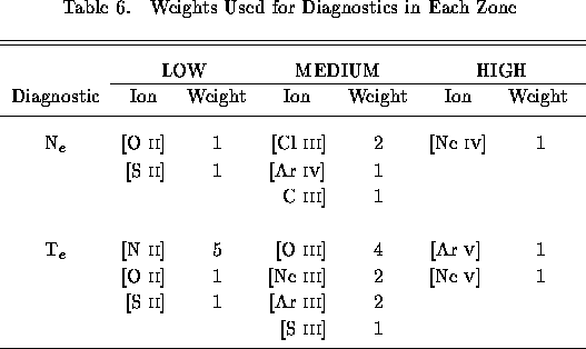
While each zone makes potential use of several diagnostics, in practice not
all diagnostics are equally reliable. The [S III]  and
and
 lines are often contaminated by atmospheric water vapor, for
example, and the auroral lines of [Ne III] and [Ar III] are often
blended with other lines. So the derived T
for the intermediate-ionization
zone is weighted toward the [O III] temperature. The weighting factors
for all the diagnostics used in the zones task are given in
Table 6 . Note that it is possible to re-derive the average N and
T for each zone using a different weighting, if desired.
lines are often contaminated by atmospheric water vapor, for
example, and the auroral lines of [Ne III] and [Ar III] are often
blended with other lines. So the derived T
for the intermediate-ionization
zone is weighted toward the [O III] temperature. The weighting factors
for all the diagnostics used in the zones task are given in
Table 6 . Note that it is possible to re-derive the average N and
T for each zone using a different weighting, if desired.
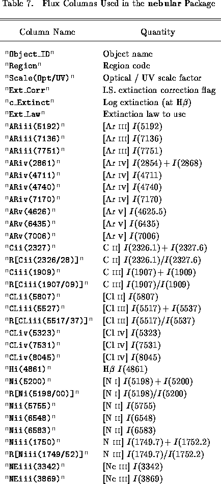
The modelling tasks also make use of the binary TABLES data structure
described above. Again, if only incomplete information is available in the
input table, the modelling tasks make use of whatever fluxes are available,
and use reasonable defaults (e.g., T = 10,000 K, N
= 1000 cm ) when necessary. In particular, any emission line
flux that is unavailable (e.g. the relevant line fluxes are ``INDEF,''
or the column name for that line flux is not found) is excluded from the
calculations. If there are no valid diagnostic line fluxes available for
a given ion, the result for that ion is INDEF, and it does not contribute
to the final average for that zone. The quantities used by the zones
task are given in Table 7 ( A and
B ) by column name.
In spite of the weighting scheme, and even if legitimate values are found for
several diagnostics, it is still possible for the average N
or T to be
skewed if there are bad data, or if the actual N or T lies outside the
range of one or more diagnostics. For this reason, the investigator should
review the output table from the zones task to ensure that the average
computed temperatures and densities are reasonable, and change them with the
table editor if they are not.
) when necessary. In particular, any emission line
flux that is unavailable (e.g. the relevant line fluxes are ``INDEF,''
or the column name for that line flux is not found) is excluded from the
calculations. If there are no valid diagnostic line fluxes available for
a given ion, the result for that ion is INDEF, and it does not contribute
to the final average for that zone. The quantities used by the zones
task are given in Table 7 ( A and
B ) by column name.
In spite of the weighting scheme, and even if legitimate values are found for
several diagnostics, it is still possible for the average N
or T to be
skewed if there are bad data, or if the actual N or T lies outside the
range of one or more diagnostics. For this reason, the investigator should
review the output table from the zones task to ensure that the average
computed temperatures and densities are reasonable, and change them with the
table editor if they are not.
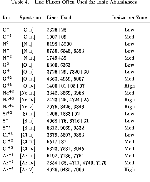
The abundances for the 3-zone model are calculated with the abund task
using the output table from zones.
The emission lines that are actually used in the 3-zone model (which are
generally also the strongest) are given in Table and N that are used for each ion are listed in Table 4
in the ``Ionization Zone'' column, although that choice can be overridden
by choosing a constant T or
N throughout the nebula. The calculated
ionic abundance is the
weighted average of that derived from each of the emission lines for that
ion, where the weight is roughly proportional to the relative line intensity.
For example, the relative weights of [O III]  are 30:10:1. Again, if no line fluxes are available for a given ion, the
computed abundance in the output table is INDEF.
are 30:10:1. Again, if no line fluxes are available for a given ion, the
computed abundance in the output table is INDEF.