Entry 11
Authors
- Robert Nikutta
Clustering of astronomical objects in WISE 3D color space
Based on: Nikutta, Hunt-Walker, Ivezic, Nenkova, Elitzur, ‘The meaning of WISE colours - I. The Galaxy and its satellites’, MNRAS 442, 3361-3379 (2014) http://dx.doi.org/10.1093/mnras/stu1087 http://adsabs.harvard.edu/abs/2014MNRAS.442.3361N
NASA’s Wide-field Infrared Survey Explorer (WISE) mapped the entire Infrared (IR) sky with unprecedented sensitivity. It produced a staggering catalog with more than half a billion objects, with precise measurements of their magnitudes in four different wavelength filters:
http://wise2.ipac.caltech.edu/docs/release/allsky/
We can learn a lot about these IR sources by studying not only their magnitudes (how bright they are), but also their colors (how much their brightness changes between filters).
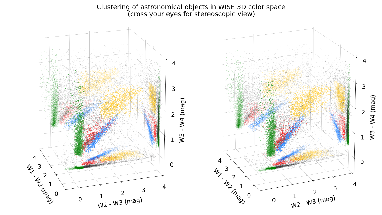
Taking for this plot from the catalog only bright objects which have robust detections (not much noise), we end up with ~15,000 sources for which we have three color measurements, W1-W2, W2-W3, W3-W4, where the ‘Wx’ are the magnitudes measured by WISE. We then plot the three colors of all 15k objects in a 3D scatter plot - every dot is one star.
Because of different physical properties, these stars tend to occupy different regions in this color-color-color (CCC) diagram. Some are so-called Asymptotic Giant Branch stars (AGB), evolving stars that are 1000 times as bright as our Sun and shrouded in layers of dust that blow away from the star like a wind, propelled by the star’s light. Depending on the dust chemistry (carbon or oxygen-rich) these shells produce different WISE colors, and so the two sub-types of AGBs separate in the CCC diagram. We plot them red (O-rich) and blue (C-rich) here. Curiously, most C-rich AGBs are found in the Large Magellanic Cloud, a beautiful small satellite galaxy of our Milky Way, which can be seen in the Southern Hemisphere with the naked eye. It is chemically quite different from our Galaxy.
Other types of stars, so called Young Stellar Objects (YSO) have different WISE colors still! In green we show YSOs which we know have thin dusty shells with constant density profiles, and are of moderate/cool temperatures (~600 Kelvin). In orange we show also YSOs, but their optical depths are larger, and their temperatures are higher (~1200 Kelvin). Other, unclassified, objects are shown as small black dots. We demonstrated in our paper
http://adsabs.harvard.edu/abs/2014MNRAS.442.3361N
how same-type objects can be identified using only WISE measurements. With this plot we demonstrate that a 3D view of the color space is necessary, because in classical 2D CC diagrams the clusters can overlap, and it is then impossible to separate them cleanly.
I used matplotlib to generate this plot. Two views of the scene are produced, offset by 5 degrees from each other in azimuthal direction. If you cross your eyes (try to see the tip of your nose) you can easily see the clusters in 3D, where everything appears extra-sharp. If you then move your head very slightly up/down or left/right, the illusion of 3D is perfect.
A function is included in the code to generate the frames of a movie, with the scene rotating in in front of the camera. You can watch the entire movie in 3D if you “cross your eyes” during the first frames of the movie.
Source
"""2015 SciPy John Hunter Excellence in Plotting Contest

Author: Robert Nikutta <robert.nikutta@gmail.com>

Title: Clustering of astronomical objects in WISE 3D color space

Based on: Nikutta, Hunt-Walker, Ivezic, Nenkova, Elitzur,
'The meaning of WISE colours - I. The Galaxy and its satellites',
MNRAS 442, 3361-3379 (2014)
http://dx.doi.org/10.1093/mnras/stu1087
http://adsabs.harvard.edu/abs/2014MNRAS.442.3361N

This stereoscopic plot (cross your eyes!) shows the distribution of
different types of astronomical objects in the 3D color space of the
WISE spacecraft (Wide-field Infrared Survey Explorer). Several classes
of objects are identified with differently colored dots. In
traditional 2D color-color plots clusters can overlap, making it
difficult to identify them. A 3D color-color plot, and especially a
stereoscopic view of it, provides a much more intuitive and immersive
experience.

Carbon-rich Asymptotic Giant Branch stars (AGB) are shown in
blue. Most of them are found in the Large Magellanic
Cloud. Oxygen-rich AGB stars are shown in red. Young Stellar Objects
(YSO) which are surrounded by dusty shells with constant radial
density profiles and small optical depths are shown in green. Both
cool (~600 Kelvin) and warm (~1200 Kelvin) shells fall in this
region. Warmer YSO shells of constant density fall in the the cluster
of orange color, but their optical depths are also higher. Finally,
small black dots show other astronomical objects in our Galaxy and its
satellites which have not been associated with the other
clusters. They are typically a mix of everything.

Example:
-------

import plot
F = plot.Figure(nxpix=1920) # full HD
F.make_stereoscopic_3d_scatter() # generates PNG file with default settings

"""

__author__ = 'Robert Nikutta <robert.nikutta@gmail.com>'
__version__ = '20150412'

import numpy as N
import pylab as p
import matplotlib
from matplotlib.gridspec import GridSpec
from mpl_toolkits.mplot3d import Axes3D


class Figure:

    def __init__(self,nxpix=1280):

        """Generate a 3D stereoscopic view of ~15k WISE sources. Color
        clusters of objects differently.

        Parameters:
        -----------
        nxpix : int
            Number of pixels of the output (PNG) file. An aspect ratio
            of 16:9 is assumed.
        """

        self.dpi = 100
        self.aspect = 16./9.

        self.ux = nxpix/float(self.dpi)
        self.uy = self.ux/self.aspect

        # Load data (WISE colors)
        print "Loading data..."
        with N.load('data.npz') as datafile:
            self.x, self.y, self.z = datafile['x'], datafile['y'], datafile['z']

        print "Number of objects: %d" % self.x.size
        print "Done."


    def make_stereoscopic_3d_scatter(self,azimuth=-18,saveformat='png'):

        """Generate two panels, 5 degrees apart in azimuth. Cross eyes for
        stereoscopic view.

        Parameters:
        -----------
        azimuth : {float,int}
            The azimuth angle (in degrees) at which the camera views
            the scene.

        saveformat : str
            Generate an output file, with the supplied azimuth in the
            file name. Must be either 'png' (recommended, default) or
            'pdf' (will be rather slow to save).

        Returns:
        --------
        Nothing, but saves an output file.

        """

        assert (saveformat in ('png','pdf')), "saveformat must be 'png' (recommended) or 'pdf' (will be very slow to save)."

        filename = '3D_color_stereoscopic_az%07.2f.%s' % (azimuth,saveformat)
        print "Generating plot %s" % filename

        self.setup_figure(figsize=(self.ux,self.uy))   # width, height

        # left panel (=right eye)
        ax1 = p.subplot(self.gs3D[0],projection='3d',aspect='equal',axisbg='w')
        plot_scatter_3D(self.fig,ax1,1,self.x,self.y,self.z,self.uy,azimuth=azimuth)

        # right panel (=left eye)
        ax2 = p.subplot(self.gs3D[1],projection='3d',aspect='equal',axisbg='w')
        plot_scatter_3D(self.fig,ax2,2,self.x,self.y,self.z,self.uy,azimuth=azimuth-5)

        if saveformat == 'png':
            p.savefig(filename,dpi=100)
        else:
            p.savefig(filename)

        p.close()


    def make_movie_frames(self,azstart=1,azstop=10,azstep=1):

        """Helper function to generate frames (for a video) with varying
        azimuth angle.

        Parameters:
        -----------
        azstart, azstop, azstep : float-ables
            The azimuth angles of first frame, last frame
            (approximate), and of the step size. All in degrees. All
            can be negative (determines direction of scene rotation)

        """

        try:
            azstart = float(azstart)
            azstop = float(azstop)
            azstep = float(azstep)
        except ValueError:
            raise Exception, "azstart, azstop, azstep must be convertible to a floating point number."

        if azstop < azstart:
            azstep = -N.abs(azstep)

        allaz = N.arange(azstart,azstop,azstep)

        for j,az in enumerate(allaz):
            print "Generating frame file %d of %d" % (j+1,len(allaz))
            self.make_stereoscopic_3d_scatter(azimuth=az)


    def setup_figure(self,figsize):

        """Set up the figure and rc params."""

        self.fontsize = 2*self.uy

        p.rcParams['axes.labelsize'] = self.fontsize
        p.rcParams['font.size'] = self.fontsize
        p.rcParams['legend.fontsize'] = self.fontsize-2
        p.rcParams['xtick.labelsize'] = self.fontsize
        p.rcParams['ytick.labelsize'] = self.fontsize

        self.fig = p.figure(figsize=figsize)  # width, height  300dpi
        self.fig.suptitle('Clustering of astronomical objects in WISE 3D color space\n(cross your eyes for stereoscopic view)',color='k',fontsize=self.fontsize+2)

        # this will hold the 3D scatter plot
        self.gs3D = GridSpec(1,2)
        self.gs3D.update(left=0.02,right=0.98,bottom=0.,top=1.,wspace=0.05,hspace=0.)


def plot_scatter_3D(fig,ax,sid,x,y,z,unit,azimuth=-25):

    # some constants
    lo, hi = -0.5, 4  # plotting limits
    s = unit/2.5      # standard marker size for scatter plot

    # conditions to select groups of objects
    coO = (x > 0.2) & (x < 2) & (y > 0.4) & (y < 2.2) & (z > 0) & (z < 1.3) & (z > 0.722*y - 0.289)      # oxygen-rich AGN stars
    coC = (x > 0.629*y - 0.198) & (x < 0.629*y + 0.359) & (z > 0.722*y - 0.911) & (z < 0.722*y - 0.289)  # carbon-rich AGN stars
    coCDSYSOcool = (x < 0.2) & (y < 0.4)                                                                 # both cool & warm YSO shells w/ constant density profile & low optical depth
    coCDSYSOwarm = (x > 0.3) & (x < 1.4) & (y > 1.4) & (y < 3.5) & (z > 1.5) & (z < 2.8)                 # warm YSO shells w/ constant density profile and high optical depth
    coOTHER = ~(coO | coC | coCDSYSOcool | coCDSYSOwarm)                                                 # other/unidentified (a mix of everything)

    groups = [coO,coC,coCDSYSOcool,coCDSYSOwarm,coOTHER]

    # plot side panes
    marker = 'o'
    colors = ('r','#1A7EFF','g','#FFC81A','0.2') # red, blue, green, orange, very dark gray
    alphas = [0.3]*len(groups)
    sizes = [s,s,s,s,s/3.]  # make 'other' apear a bit less prominent
    for j,group in enumerate(groups):
        cset = ax.scatter(x[group], y[group], lo, zdir='z', s=sizes[j], marker=marker, facecolors=colors[j], edgecolors=colors[j], linewidths=0., alpha=alphas[j])
        cset = ax.scatter(y[group], z[group], hi, zdir='x', s=sizes[j], marker=marker, facecolors=colors[j], edgecolors=colors[j], linewidths=0., alpha=alphas[j])
        cset = ax.scatter(x[group], z[group], hi, zdir='y', s=sizes[j], marker=marker, facecolors=colors[j], edgecolors=colors[j], linewidths=0., alpha=alphas[j])

    # plot 3D clusters
#    labels = ['O-rich AGB','C-rich AGB',r'cool YSO shells, $\rho(r)$=const.',r'warm YSO shells, $\rho(r)$=const., high optical depth','other']
    alphas = [0.8,0.8,0.8,0.8,0.4]  # make 'other' apear a bit less prominent
    for j,group in enumerate(groups):
        ax.scatter(x[group], y[group], z[group], s=sizes[j], marker=marker, facecolors=colors[j], edgecolors='w', linewidths=0.1, alpha=alphas[j])

    # generate view
    ax.view_init(elev=18, azim=azimuth)

    # per-axis settings
    for prop in ('w_xaxis','w_yaxis','w_zaxis'):
        obj = getattr(ax,prop)
        obj.set_pane_color((1,1,1,1.0))
        obj.gridlines.set_lw(0.3)
        obj._axinfo.update({'grid' : {'color': (0.5,0.5,0.5,1)}})


    # final touch ups
    ax.set_xlim(hi,lo)
    ax.set_ylim(lo,hi)
    ax.set_zlim(lo,hi)

    ax.set_xticks((0,1,2,3,4))
    ax.set_yticks((0,1,2,3,4))
    ax.set_zticks((0,1,2,3,4))

    ax.set_xlabel('W1 - W2 (mag)')
    ax.set_ylabel('W2 - W3 (mag)')
    ax.set_zlabel('W3 - W4 (mag)')