Entry 1

Authors

• Alex J. DeCaria

Abstract

Spectral analysis is the process of decomposing a signal or function into a sum of orthogonal basis function of differing amplitudes. A familiar form of spectral analysis is Fourier analysis in which the basis functions are sines and cosines, and the signal is decomposed into a sum of sines and cosines of specific amplitudes and wavelengths. The amplitudes are called the spectral coefficients of the signal.

For spherical domains the coordinates are latitude (\(\varphi\)) and longitude (\(\lambda\)), and the basis functions are not pure sines and cosines. Instead, more complicated basis functions called spherical harmonics are used. Spherical harmonics have the mathematical form:

\[Y_{m,n}(\mu, \lambda) = \sqrt{\frac{(2n+1)(n-m)!}{(n+m)!}}P_{m,n}(\mu)e^{m \lambda}\]

where \(\mu = sin \varphi\), and \(P_{m,n}\) is the associated Legendre function of the first kind with order \(m\) and degree \(n\). The order and degree are both integers, and have the following restrictions:

\[-\infty \leq m \leq \infty\]

\[n - |m| \geq 0\]

The spherical harmonics are complex-valued functions, having both a real and an imaginary component. On the globe a scalar field such as pressure, \(p(\mu, \lambda)\) , can be represented as a sum of spherical harmonics,

\[p(\mu, \lambda) = \sum_{m=-\infty}^{\infty} \sum_{n=|m|}^{|m|+M} H_{m,n} Y_{m,n}\]

where the \(H_{m,n}\) are the complex amplitudes, or spectral coefficients, of the function \(p(\mu, \lambda)\).

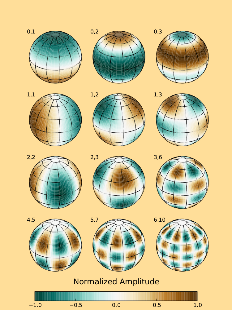
The figure illustrates normalized plots of the real component, \(Re[Y_{m,n}]\), of several spherical harmonics of various order and degree. The order, \(m\), corresponds to the number of null (zero- valued) circles that pass through the poles. The value \(n − |m|\) corresponds to the number of null circles that are parallel to the latitude lines. For example, in the plot for \((m, n) = (5, 7)\) there are five null circles running through the poles and 2 null circles running parallel to the equator. The plot was generated using Python, numpy, Matplotlib, Basemap, and the ‘special’ module from Scipy.

Spherical harmonics have applications in many physical problems with spherical geometry. One such application is in global numerical modeling of the atmosphere, in which atmospheric variables are decomposed into their spectral components. This figure is based on Figure 11-2 from the book A First Course in Atmospheric Numerical Modeling, by Alex J. DeCaria and Glenn E. Van Knowe, published in 2014 by Sundog publishing. As an interesting aside, most of the numerous illustrations in this book were generated using Python, Numpy, and Matplotlib.

Products

• PDF

Source

• IPython notebook (ipynb)