Entry 20
Authors
- Konstantin Fedotov
Products
Galaxies like our Milky Way are collections of hundreds of billions of stars and giant clouds of gas from which new stars can be born. When galaxies crash into other galaxies, gravity can compress these clouds, triggering a burst of new stars. The gas can also be pulled out from galaxies into large tidal features – streams of stars and gas that have been “sheared off” from the outskirts of their parent galaxies. At times, the tidal streams can also host vigorous star formation that can be seen for up to a billion years after it starts. This is precisely the case for the two galaxies featured on the image, which are in the midst of a high speed (900 km/s!) collision.
This pair is part of a small group of galaxies known as Stephan’s Quintet located almost 300 million light years away. At this distance, we cannot separate individual stars. Instead, we detect and study star clusters, very compact groups of a few thousand up to a few million stars that were all born at the same time from the same cloud of gas. On the image, an entire star cluster appears as a single point. Using multicolor images with the Hubble Space Telescope, we were able to estimate the ages and masses of individual star clusters throughout the interacting pair of galaxies.
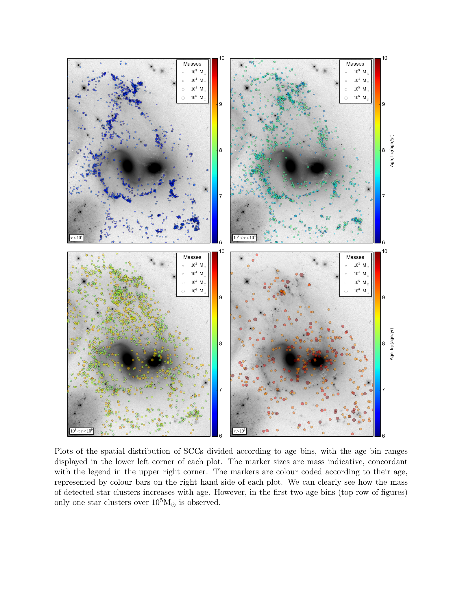
The four-panel plot features HST images of the galaxies as a background with the locations of star clusters superimposed. Each panel shows only the star clusters in a limited age range. Each cluster is represented by a circle whose radius is scaled by the mass of the cluster (according to the legend in the upper right corner) and the color of the circle represents the cluster’s age (according to the color bar on the right hand side of each plot). Comparing star clusters between the different regions observed in the image, we find that the youngest clusters are very tightly concentrated in all the regions, while clusters with older ages are more distributed. Moreover, we observe a significantly larger number of clusters with ages over 10 million years outside of the galaxies. This indicates that either star formation has been proceeding in the space between the galaxies for a while now, or that the older clusters were stripped from the host galaxies (or some combination of the two). Another striking featured discovered by studying the images is that there are no massive young clusters (larger than 100 thousand solar masses). The current environment is apparently suppressing the formation of massive clusters.
To have a better feel for the dynamics of star formation, we also created a short animation that shows the spatial map of clusters formed in the last 30 million years. The animation illustrates the progression of star formation over time more clearly than the static images; the intensity of star formation is increasing significantly as we move closer to the present time. As an example, a brief burst of star formation in the Southern Debris region (lower right corner of the image) pops out in the animation at t~300 thousand years.
Overall, this star cluster study allows us to date epochs of star formation in Stephan’s Quintet triggered by galaxy interactions.
For more information about this plot please see my Ph.D. thesis,.
Source
# -*- coding: utf-8 -*-
"""
Created on Fri Apr  3 22:22:57 2015

Code creates animated map of star clusters formation in Stephan's Quinted.

@author: kfedotov
"""
from moviepy.video.io.bindings import mplfig_to_npimage
from matplotlib.ticker import LinearLocator
from matplotlib.colors import LogNorm
from moviepy.editor import VideoClip
import matplotlib.pyplot as plt
from astropy.io import ascii
import numpy as np
import pyfits
import pylab

#  Load data
data = ascii.read('final_catalog.cat', Reader=ascii.CommentedHeader, comment='#', guess=False)

#  Set the upper age level
up_age = 10**7.5

#  Read FITS image
f = pyfits.open('sq2.fits')
im = f[0].data

#  Set size and plot the image
fig = plt.figure(figsize=(6.25, 6.5), tight_layout=True)
ax = fig.add_subplot(111)
ax.imshow(im,
          cmap=pylab.cm.gist_yarg,
          norm=LogNorm(vmin=125,vmax=2500),
          aspect='equal')
plt.tight_layout()

#  Remove labels from scatter plot
#  Rotate image
ax.get_yaxis().set_visible(False)
ax.get_xaxis().set_visible(False)
ax.set_ylim(2, im.shape[0]-2)
ax.set_xlim(2, im.shape[1]-2)

#  Plot colorbar
cm = plt.cm.cool
sm = plt.cm.ScalarMappable(cmap=cm,
                           norm=plt.Normalize(vmin=0.1, vmax=up_age/10**6))
sm.set_array([])
cbar = plt.colorbar(sm,
                    ticks=LinearLocator(),
                    format="%1.0f",
                    drawedges=False,
                    pad=0.01,
                    aspect=25)
cbar.set_label(r'Age, Myr', fontsize=14)
cbar.ax.tick_params(labelsize=14)

# Resetting color scale for clusters
sm = plt.cm.ScalarMappable(cmap=cm,
                           norm=plt.Normalize(vmin=10**5, vmax=up_age))
#  Import WCS info
from astropy.wcs import WCS
w = WCS('sq2.fits')

#  Filter star clusters for chosen time interval
yr_age = data['age']
ind, = np.where(yr_age < up_age)
age = yr_age[ind]
x, y = w.wcs_world2pix(data['RA'][ind], data['Dec'][ind], 0)

#  Setting up scheeme for SCC size
ms = data['log_mass'][ind]
size = ms * np.log2(ms)**2*2

#  Setting up parameters printing
#log_time = plt.text(100, 200, '0', fontsize='14')
time = plt.text(100, 100, '0', fontsize='14')

#  Setting up temporary variables
res = ax.scatter([], [])
ar, wght, alp = [], [], []

def make_frame(t):
  global curr, ar, wght, alp, res
  i, = np.where((age <= curr) & (age > curr - step))
  if len(i):
    ar.extend(l for l in i)
    wght.extend(0 for l in i)
    alp.extend(1.0 for l in i)
  # adjust the weights, so that the points appear gradually
  weights = np.minimum(1, np.maximum(0, np.array(wght)+0.1))
  # adjust the alpha, so that the older points gradually faint away
  sm.set_array(age[ar])
  rgba = sm.to_rgba(age[ar])
  rgba[:, 3] = np.maximum(0.075, alp)
  if len(ar):
    res.remove()
    res = ax.scatter(x[ar], y[ar],
                     c=rgba,
                     s=np.array(size[ar]*weights),
                     linewidth=np.array(0.75*np.maximum(0.075, alp))
                     )
  #log_time.set_text('{num:0.3f}'.format(num=np.log10(curr)) + ' log(yr)')
  time.set_text('{num:0.3f}'.format(num=curr/10**6) + ' Myr')
  wght = [n + 0.2 for n in wght]
  alp = [n - st for n in alp]
  curr = curr - step
  return mplfig_to_npimage(fig)

#  Setting up movie parameters (length in sec, fps)
D = 30.
fps = 40.

#  Step in age, initiate current age, and parameter controloing the speed of
#  point fainting
step = round(max(age) - min(age), 3) / D / fps
curr = round(max(age), 3)
st = 40./len(ind)

#  Calling animation
animation = VideoClip(make_frame, duration = D)

#  Mass legend
l1 = plt.scatter([],[], s=3*np.log2(3)**2*2, c='w', linewidths=0.5)
l2 = plt.scatter([],[], s=4*np.log2(4)**2*2, c='w', linewidths=0.5)
l3 = plt.scatter([],[], s=5*np.log2(5)**2*2, c='w', linewidths=0.5)
l4 = plt.scatter([],[], s=6*np.log2(6)**2*2, c='w', linewidths=0.5)
label = [r'$10^3$ M$_{\odot}$',
         r'$10^4$ M$_{\odot}$',
         r'$10^5$ M$_{\odot}$',
         r'$10^6$ M$_{\odot}$']
legend = plt.legend([l1, l2, l3, l4],
                    label,
                    frameon=True,
                    loc = 1,
                    prop={'size':14},
                    bbox_to_anchor=[.999, .999],
                    borderpad = .25,
                    title='Masses',
                    scatterpoints = 1)
plt.setp(legend.get_title(),fontsize='14')

#  Write gif file
animation.write_gif('SQ_movie_linear.gif',
                    fps=fps,
                    program='ImageMagick',
                    opt='OptimizeTransparency')
# -*- coding: utf-8 -*-
"""
Created on Thu Oct 30 15:59:34 2014

Plots of star clusters age spatial distribution for certain mass ranges

@author: kfedotov

"""

# Import necessary modules
from mpl_toolkits.axes_grid1 import make_axes_locatable
from matplotlib.ticker import MultipleLocator
from matplotlib.colors import LogNorm
import matplotlib.pyplot as plt
from astropy.io import ascii
import numpy as np
import pyfits
import pylab


def plot_distr(data, ind, j):
  #  Read FITS image
  f = pyfits.open('sq2.fits')
  im = f[0].data

  #  Generate initial figure, scatter plot, and histogram quadrants
  fig = plt.figure(figsize=(6, 8))
  axScatter = fig.add_subplot(111)

  #  Plot the image
  axScatter.imshow(im,
                   cmap=pylab.cm.gist_yarg,
                   norm=LogNorm(vmin=150,vmax=2500),
                   aspect='equal')

  #  Remove labels from scatter plot
  axScatter.get_yaxis().set_visible(False)
  axScatter.get_xaxis().set_visible(False)

  #  Rotate image
  axScatter.set_ylim(2,im.shape[0]-2)
  axScatter.set_xlim(2,im.shape[1]-2)

  #  Import WCS info
  from astropy.wcs import WCS
  w = WCS('sq2.fits')
  x, y = w.wcs_world2pix(data['RA'][ind], data['Dec'][ind], 0)

  #  Setting up scheemes for SCC size, transparency, and color
  ms = data['log_mass'][ind]
  size = ms * np.log2(ms)**2
  trans = 100 - 100*data['mass'][ind]/max(data['mass'][ind])
  z = np.array(data['log_age'][ind])
  cm = plt.cm.get_cmap('jet')

  #  Plot SCCs
  for i in range(len(ind)):
    sc = axScatter.scatter(x[i], y[i],
                           marker='o',
                           s=size[i],
                           c=z[i],
                           cmap=cm,
                           vmin=6,
                           vmax=10,
                           alpha=0.45,
                           zorder=trans[i],
                           linewidths=0.5)

  #  Plot colorbar
  divider = make_axes_locatable(axScatter)
  cax = divider.append_axes("right", size="4%", pad=0.05)
  cbar = plt.colorbar(sc,
                      cax=cax,
                      ticks=MultipleLocator(1.),
                      format="%1.f",
                      drawedges=False)
  if j in [1, 3]:
    cbar.set_label(r'Age, $\log($age$/$yr$)$', fontsize=10)
  cbar.set_alpha(1)
  cbar.draw_all()

  #  Mass legends
  l1 = plt.scatter([],[], s=3*np.log2(3)**2, c='w', linewidths=0.25)
  l2 = plt.scatter([],[], s=4*np.log2(4)**2, c='w', linewidths=0.25)
  l3 = plt.scatter([],[], s=5*np.log2(5)**2, c='w', linewidths=0.25)
  l4 = plt.scatter([],[], s=6*np.log2(6)**2, c='w', linewidths=0.25)
  label = [r'$10^3$ M$_{\odot}$',
           r'$10^4$ M$_{\odot}$',
           r'$10^5$ M$_{\odot}$',
           r'$10^6$ M$_{\odot}$']
  plt.legend([l1, l2, l3, l4],
             label,
             frameon=True,
             loc = 1,
             prop={'size':10},
             bbox_to_anchor=[-0.2, 1.005],
             borderpad = .5,
             title='Masses',
             scatterpoints = 1)
  label = [r'$\tau < 10^7$',
           r'$10^7\!< \tau < 10^8$',
           r'$10^8\!< \tau < 10^9$',
           r'$\tau > 10^9$']
  axScatter.annotate(label[j],
                     xy=(60, 75),
                     textcoords='data',
                     fontsize=10,
                     bbox=dict(fc='white', ec='k'),
                     zorder=99)
  ttls = ['SciPy_age_distr_bin1',
           'SciPy_age_distr_bin2',
           'SciPy_age_distr_bin3',
           'SciPy_age_distr__bin4']
  plt.savefig(ttls[j]+'.png',
              bbox_inches='tight',
              format='png',
              pad_inches=0.05,
              dpi=200)
  return


#  Load data
#  Columns: RA, Dec, chi, ebv, age, mass, vmag, vmagerr, id, label
data = ascii.read('final_catalog.cat',
                  Reader=ascii.CommentedHeader,
                  comment='#',
                  guess=False)

#  Initiallizing array-holders
ind = [[0 for x in xrange(1)] for x in xrange(4)]

#  Distribute clusters according to their ages

ind[0], = np.where(data['log_age'] <= 7)
ind[1], = np.where( (data['log_age'] > 7) & (data['log_age'] <= 8) )
ind[2], = np.where( (data['log_age'] > 8) & (data['log_age'] <= 9) )
ind[3], = np.where(data['log_age'] > 9)

#  Call plotting routine
for i in xrange(4):
  plot_distr(data, ind[i], i)