Entry 8

Authors

• Hywel Farnhill

Astronomical surveys allow the study of large areas of the sky down to extremely faint limiting magnitudes. Using the Isaac Newton Telescope on La Palma, the INT Photometric H-alpha Survey of the Northern Galactic Plane (IPHAS) provides a catalogue of 219 million stars, observed in two broad-band filters (r and i) and the narrow-band H-alpha.

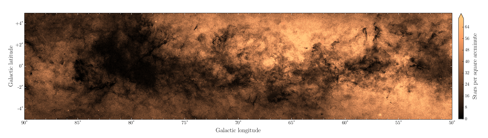
Such a large-scale survey can enable the measuring of stellar density across the Galactic Plane, however effects of crowding and incompleteness lead to a certain fraction of stars being missed. Measures of stellar densities corrected for these effects would be useful for testing the predictions of models of Galactic populations. By utilising 62,000 hours of processing time on the HPC facility at the University of Hertfordshire’s Science and Technology Research Institute, the impact of crowding was assessed for each of the 14,115 fields included in the latest data release of IPHAS. This allowed the incompleteness of each field to be quantified, providing the corrections necessary to obtain stellar densities across the Northern Galactic Plane.

This map visualises the corrected stellar density of stars down to 19th magnitude in the redder i-band, at a resolution of 1 x 1 square arcminute, for a 400 square degree region of the Galactic Plane. The copper colour scheme was chosen to depict stellar density in order to provide contrast while remaining a recognisable reproduction of the naked-eye night sky. The chosen region highlights the range of densities observed, an effect caused by the obscuration of sources by interstellar dust - particularly evident is the Cygnus-X molecular cloud complex around longitude 80°. A number of star clusters are visible as small-scale overdensities.

Where IPHAS is data is unavailable across this region, or bright stars have been masked out, the star counts have been interpolated - this amounts to 2% of the mapped area.

Products

• PDF

Source

import numpy as np
import matplotlib.pyplot as plt
from matplotlib.ticker import FuncFormatter as Fmt

# Matplotlib settings for a nice looking plot
plt.rcParams['text.latex.unicode'] = True
plt.rcParams['text.usetex'] = True
plt.rcParams['font.family'] =  'serif'
plt.rcParams['font.serif'] =  'Computer Modern'

# Format latitude tick labels nicely
def latitude(b, pos):
    if b > 0:
        return u"+{0:.0f}\u00b0".format(b)
    else:
        return u"{0:.0f}\u00b0".format(b)

# Import the data and plot it
dmap = np.load('dmap.npy')
# dmap = np.load('dmap_cutdown.npy')
fig = plt.figure(figsize=(22,6.25))
ax = fig.add_subplot(111)
im = ax.imshow(dmap, origin='lower', extent=[50, 90, -5, 5], 
               vmax=70, cmap='copper', interpolation='nearest')
#im = ax.imshow(dmap, origin='lower', extent=[50, 70, -5, 5], 
#               vmax=70, cmap='copper', interpolation='nearest')

# Extent and labelling of axes
ax.set_ylim(-5,5)
ax.set_xlim(50,90)
ax.invert_xaxis()
ax.set_xlabel('Galactic longitude', fontsize=20, labelpad=10)
ax.set_ylabel('Galactic latitude', fontsize=20)

# Formatting of axes' ticks
ax.xaxis.set_major_formatter(plt.FormatStrFormatter(u"%d\u00b0"))
ax.yaxis.set_major_formatter(Fmt(latitude))
ax.xaxis.set_minor_locator(plt.MultipleLocator(base=1.0))
ax.yaxis.set_minor_locator(plt.MultipleLocator(base=1.0))
ax.tick_params(axis='both', which='major',
               labelsize=16, color='#ffffff', size=5)
ax.tick_params(axis='both', which='minor', color='#ffffff', size=2.5)

# Colourbar
cbar = plt.colorbar(im, fraction=0.0115, pad=0.015, 
                    label=r"Stars per square arcminute", extend='max')
cbar.set_label("Stars per square arcminute", fontsize=20, labelpad=10)
cbar.ax.tick_params(labelsize=15)
cbar.solids.set_rasterized(True)

# Adjust plot size and save
plt.subplots_adjust(top=0.99, bottom=0.05, right=0.95, left=0.05)
fig.savefig('density_map.pdf')

• dmap_cutdown.npy