

The STSDAS synphot tasks allow you to:
The instrument mode sensitivity curves are generated at runtime by a passband generator by combining the throughput curves for the individual optical components that make up a given instrument observing mode. This is necessary because the number of possible instrument modes is so large that it would be impractical to independently calibrate and store the final sensitivity curves for every mode. To specify an instrument mode in the synphot tasks, you provide a list of component keywords such as WFC,3,f555w. The passband generator follows a path through the instrument graph table--i.e., the table that defines which optical components can be connected together. If the keywords define a unique path through the instrument graph, then a passband is built up as the product of the individual passbands of the components contained in the path.
The tasks graflist, grafplot, grafcheck, and grafpath are useful for getting information about a given instrument graph table. graflist makes a list of the components downstream from a given component and grafplot similarly provides a graphical representation of component paths. The grafpath task makes a list of all the component throughput tables encountered along the path of a given observation mode, while grafcheck is used to check an instrument graph table for bad rows.
Using the synphot tasks calcband or plband, you can calculate and display the sensitivity curve (passband) for any HST observing mode. These tasks also allow you to synthesize arbitrary passbands from analytic forms such as Gaussians, rectangular boxes, and series of Legendre polynomials, where you specify relevant parameters such as the central wavelengths, widths, and polynomial coefficients.
Similarly, the tasks calcspec and plspec are used to manipulate and display spectral data. The spectral data may be read from existing data files such as the HST calibration target spectral library or your own observations of targets of interest. Alternatively, spectra may be synthesized at runtime from a choice of available forms including black body, powerlaw, and HI emission spectra, where the user specifies desired parameters such as temperature, spectral slope, column density, etc. The spectrum calculator also allows you to renormalize spectra to any desired flux level, add or remove extinction effects, add and subtract spectra, and multiply by a chosen observation mode passband. Spectral data may also be calculated or converted to any of eleven types of units, including fn, fl, counts, observed magnitudes, Jy, and mjy.
The calcphot and countrate tasks can calculate photometric quantities for given combinations of spectra and observing modes. The calcphot task can be used to compute the total flux in a given passband, while the countrate task will in addition create an output spectrum containing the number of counts as a function of wavelength within the specified passband and is therefore especially well-suited for simulating observations for spectroscopy instruments, such as the Faint Object Spectrograph (FOS) and the Goddard High-Resolution Spectrograph (GHRS). The input parameters for the countrate task were specifically designed to mimic the list of entries that an observer will encounter on an HST exposure log sheet. On page 139 we provide an example of how the countrate task can be used with GHRS data.
The task plratio displays the ratio of observed to predicted photometry and spectrophotometry and produces statistics of the observations. The pltrans task displays photometric transformation plots, such as color-magnitude or color-color diagrams.
All synphot tasks are designed to read input data (for either passband throughput curves or spectral data) from tables. These input tables may be in either ASCII text format or in STSDAS table format. Output data generated by the synphot tasks are stored in STSDAS tables. The task imspec can be used to convert spectral data from IRAF or STSDAS images into STSDAS tables (or vice versa) for use in synphot.
There are several spectral atlases of observed and model data that are available in STSDAS table format for use with synphot tasks. These atlases are available from STEIS under the cdbs directory. Detailed descriptions and locations of these atlases can be found in Appendix B (page 93) of the Synphot User's Guide.
Tasks in the synphot Package
The cenwave parameter specifies the central wavelength for the simulated observation, in Angstroms; the output spectrum will be centered at this wavelength. If set to "INDEF", the output spectrum will contain the entire wavelength range covered by the chosen observation mode. This parameter only affects HRS instrument modes, because it is the only instrument where the detector cannot cover the entire wavelength range of an observation. This parameter is ignored for all non-HRS instrument modes.
The target spectrum may be specified in one of two ways:
Functional Forms
The synmag parameter is used in conjunction with synspec to normalize the synthetic spectrum to a chosen absolute flux level. This is done by specifying the desired integrated broadband magnitude, in units of stmag , for the spectrum in one of the standard UBVRI passbands. The syntax used to specify synmag is a two-word string consisting of the desired magnitude value, followed by the name of the desired passband, e.g., "synmag = 17.3 V."
In addition to computing the total counts integrated over the chosen instrument passband, it is possible to compute the number of counts at a particular reference wavelength through the use of the refwave parameter. If the chosen instrument is a spectrograph (FOS or HRS), the task will compute the counts in the pixel containing the reference wavelength. If the chosen instrument is not a spectrograph, the task will compute the counts per Angstrom at the chosen reference wavelength.
The reddening parameter may be used to add or remove the effects of interstellar reddening on the input spectrum and is specified in units of E(B - V). It provides the same functionality as the ebmv function in the spectrum interpreter of other synphot tasks. Either the user spectrum (userspec) or the synthetic spectrum (synspec) may be modified by this parameter.
The exptime parameter is used to specify the desired exposure time, in seconds, to be applied in the calculation of the total counts.
If the verbose parameter is set to "yes", then the results of the total counts and counts at the reference wavelength calculations will be written to the terminal. In addition, these two quantities are also written to the two output parameters count_tot and count_ref.
With verbose=yes, the output on your screen will be the following:
Generated with WebMaker

Example of Using countrate
To give you a feel for how synphot tasks work, we provide below a simple example of using the
countrate task. Many other examples of using synphot tasks are provided in Chapter 3 of the Synphot User's Guide. The countrate parameters are shown in Figure 6.2. Before we jump into the example, let's first look at the task first to get an idea of how synphot tasks and their parameters work.
output =            Output table name
instrument =        Science instrument
(detector = " ")    Detector used
(spec_elem = " ")   Spectral elements used
(aperture = " ")    Aperture / field of view
(cenwave = INDEF)   Central wavelength (HRS only)
(userspec = " ")    User supplied input spectrum
(synspec = " ")     Synthetic spectrum
(synmag = " ")      Magnitude of synthetic spectrum
(refwave = INDEF)   Reference wavelength
(reddening = 0.)    Interstellar reddening E(B-V)
(exptime = 1.)      Exposure time in seconds
(verbose = yes)     Print results to STDOUT ?
(count_tot = INDEF) Estimated total counts (output)
(count_ref = INDEF) Estimated counts at reference wavelength
(refdata = "")      Reference data
Countrate Task Parameters About countrate
Unlike other synphot tasks in which the observing mode is specified via the single parameter obsmode, the countrate task uses separate instrument, detector, spec_elem, and aperture parameters to specify the observing mode. The instrument parameter specifies one of the HST instruments: FGS, FOC, FOS, HRS, HSP, WF/PC, or WF/PC-2. If you set the instrument parameter to HRS, you should also specify a value for cenwave, the central wavelength of the spectrum (see below). The detector parameter specifies the name of the desired detector, if there is more than one available for the chosen instrument. The spec_elem parameter specifies the name of spectral elements, such as filters or gratings. Finally, the aperture parameter specifies the name of the instrument aperture, if there is more than one available for the chosen instrument. The instrument parameter must always be specified, but one or more of the detector, spec_elem, and aperture parameters may be left blank, depending on their applicability to a given instrument. The task automatically chooses a wavelength set tailored to each HST instrument and observing mode.
The synthetic spectrum will only be used if the userspec parameter is blank. The crcalspec$ and crgrid$ directories contain tables of HST flux calibration star spectra and various spectral atlases (both models and observational data) that can be used as source spectra. The synspec parameter recognizes the functional forms listed in Table 6.3.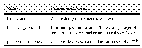
Sample countrate Run
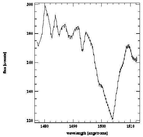
This example computes the result of a 100 second observation of the star Feige 110, using the HRS with the large science aperture (lsa) and the g160m grating. We'll also have it compute the number of counts in one pixel at 1504 Å. The spectral data for Feige 110 are read from the table feige110_002.tab in the directory crcalspec$. The calculated spectrum, in units of counts per pixel, is written to the table hrsobs.tab.
133605.84 # Total counts
   222.53 # Counts at reference pixel
Figure 6.3 shows the resulting spectrum as plotted using the STSDAS task stplot.sgraph (e.g., sgraph "hrsobs wavelength flux").
Plot of Countrate Example Spectrum